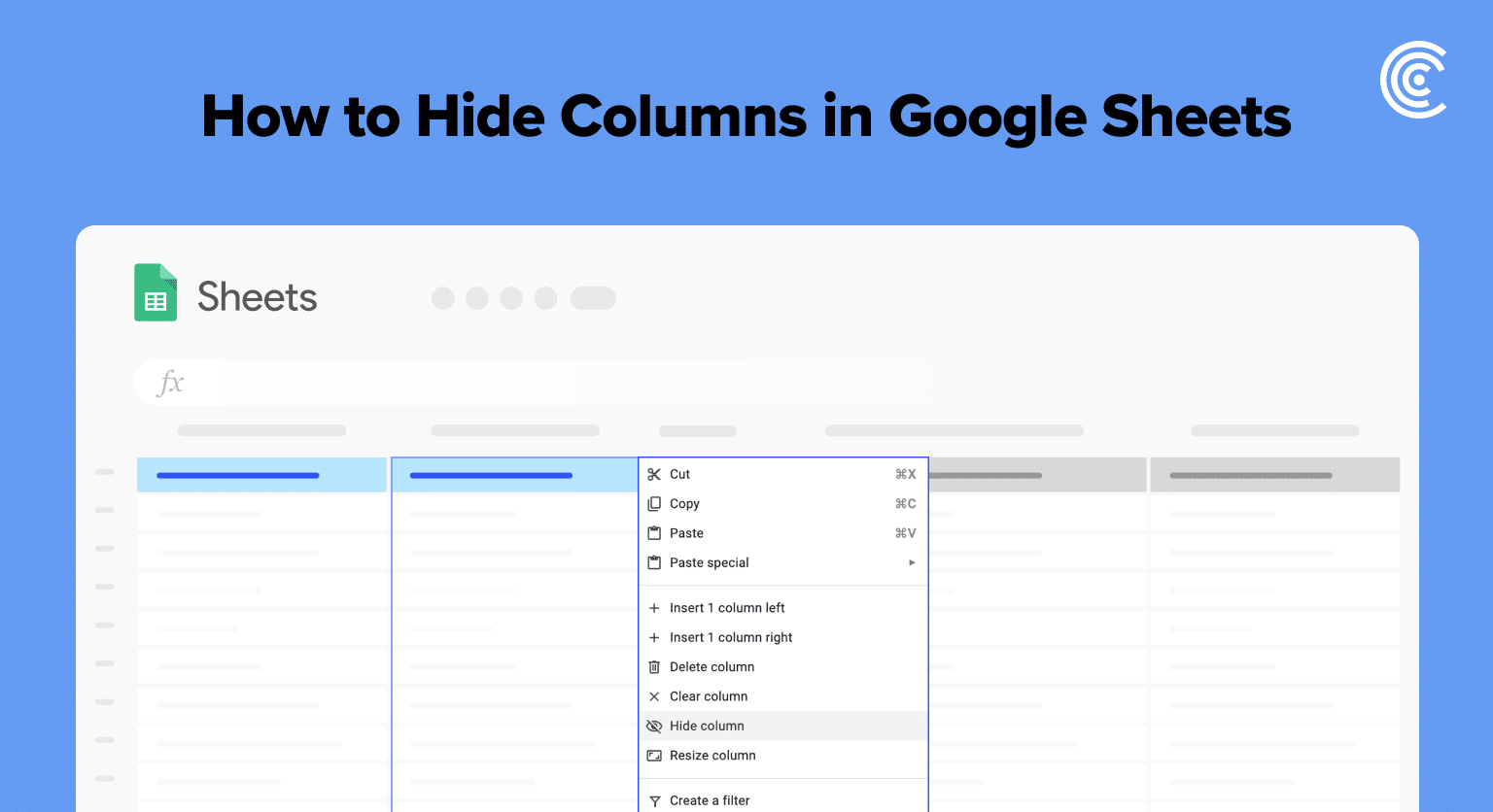
Select the column header by clicking on the column letter
Right-click on the column header and select “Hide column” from the drop-down menu
Alternatively, use keyboard shortcut “Ctrl+Alt+0” (Windows) or “Cmd+Alt+0” (Mac) to hide the selected column
For multiple adjacent columns, click and drag across column headers or use Shift+click to select a range
To unhide columns, right-click any column header and select “Unhide column” or use “Ctrl+Shift+0” (Windows) or “Cmd+Shift+0” (Mac)
If you need to unhide a column, you can do so by right-clicking on any column header and selecting “Unhide column” from the menu. You can also use the keyboard shortcut “Ctrl+Shift+0” on Windows or “Cmd+Shift+0” on Mac. It’s important to note that hidden columns will still be included in any formulas or calculations in the sheet, so be careful when hiding columns that are being used in calculations.
Basic Steps to Hide Columns in Google Sheets
Using the Right-Click Menu
One way to hide columns in Google Sheets is to use the right-click menu. Here are the steps:
- Select the column(s) you want to hide by clicking on the column letter(s) at the top of the sheet.
- Right-click on the selected column(s).
- From the drop-down menu, select “Hide column”.
Utilizing the Hide Option in the Menu Bar
Another way to hide columns in Google Sheets is to use the “Hide column” option in the menu bar. Here are the steps:
- Select the column(s) you want to hide by clicking on the column letter(s) at the top of the sheet.
- Click on the “Format” menu in the menu bar.
- Hover over “Hide & Unhide” in the drop-down menu.
- Click on “Hide columns”.
Using the Hide Option with Keyboard shortcuts
It is worth noting that you can also use keyboard shortcuts to hide columns in Google Sheets. For example, on a Windows computer, you can press “Ctrl + Alt + 0” to hide the selected column(s). On a Mac, you can press “Command + Option + 0”.
In conclusion, hiding columns in Google Sheets is a simple process that can make your data more organized and easier to analyze. By following the steps outlined above, you can quickly and easily hide columns in your Google Sheets documents.
How to hide adjacent columns in Google Sheets?
If you want to hide multiple adjacent columns, you can click and drag your mouse over the column headers to select them. Alternatively, you can click on the first column header, hold down the Shift key, and then click on the last column header to select them all.
Once you have selected the columns you want to hide, you can right-click on any of the selected column headers and choose “Hide columns X-X” from the context menu. This will hide all of the selected columns at once.
How to hide non-adjacent columns in Google Sheets?
If you want to hide non-adjacent columns, you can hold down the Ctrl key (Windows) or Command key (Mac) and click on the column headers you want to hide. You can select as many non-adjacent columns as you want.
Once you have selected the columns you want to hide, you can right-click on any of the selected column headers and choose “Hide columns X-X” from the context menu. This will hide all of the selected columns at once.
Leverage AI to Build Google Sheets Formulas, Pivots, and Charts
If you’d like to learn more about unhiding columns or managing columns on mobile devices, you’ll find a full walkthrough below.
However, if you find yourself landing on Google Sheets tutorials like this one often, leveraging AI could be a huge time-saver for you.
You can use Coefficient’s free GPT Copilot to automatically create Google Sheets formulas, pivots, and charts for you.
First, you’ll need to install the free Google Sheets Extension. You can get started with GPT Copilot here.
After you submit your email, follow along, and accept the prompts to install. Once the installation is finished, navigate to Extensions on the Google Sheets menu. Coefficient will be available as an add-on.
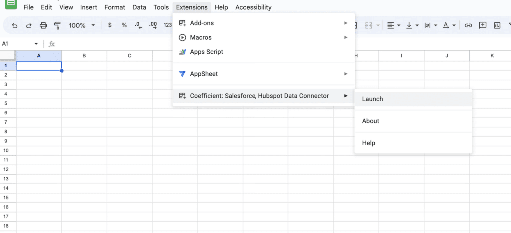
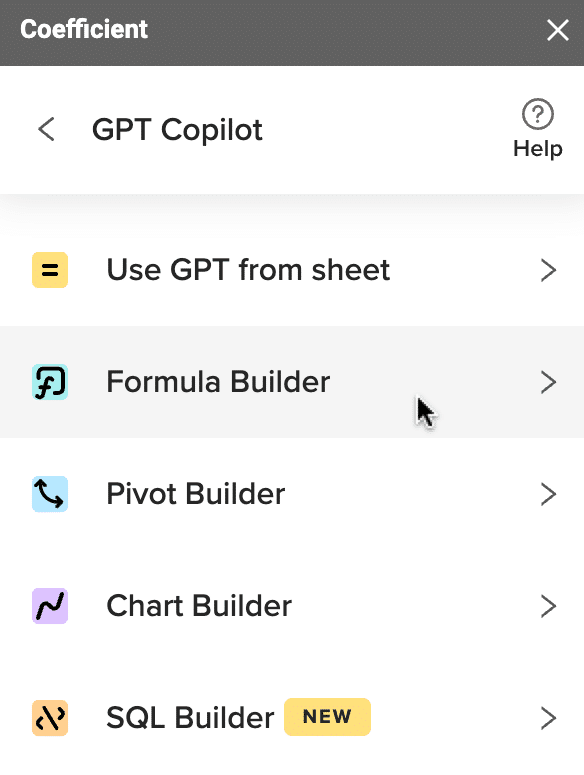
Now launch the app. Coefficient will run on the sidebar of your Google Sheet. Select GPT Copilot on the Coefficient sidebar.

For this example, we’ll use Formula Builder.

Supercharge your spreadsheets with GPT-powered AI tools for building formulas, charts, pivots, SQL and more. Simple prompts for automatic generation.

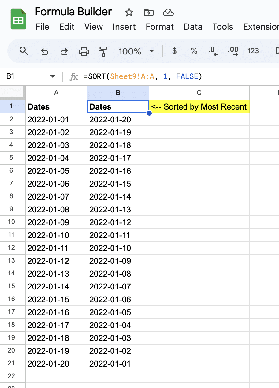
Let’s type a formula description into the text box. For this example, let’s sort 20 dates starting with the most recent date.
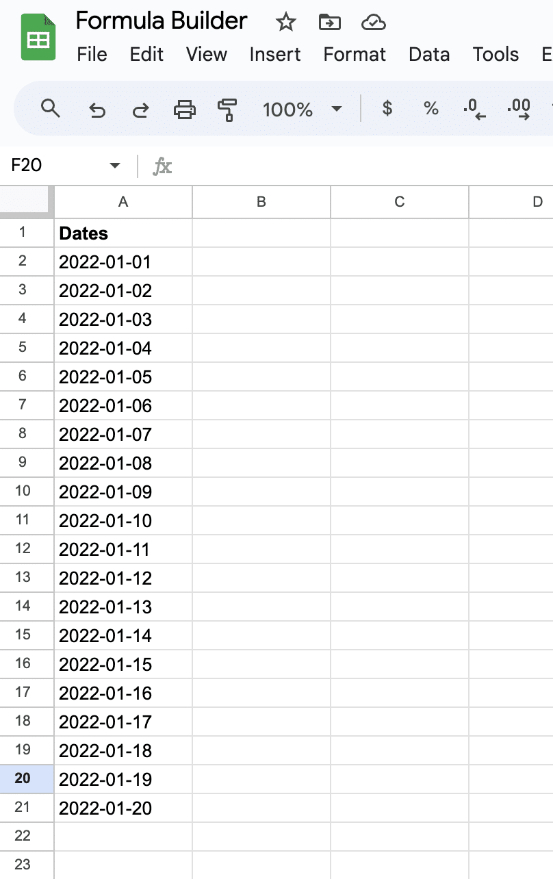
Simply type: Sort dates in column A in sheet9 by most recent date.
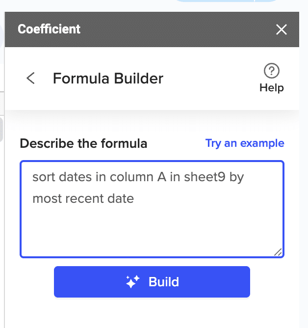
Then press ‘Build’. Formula Builder will automatically generate your sort formula.
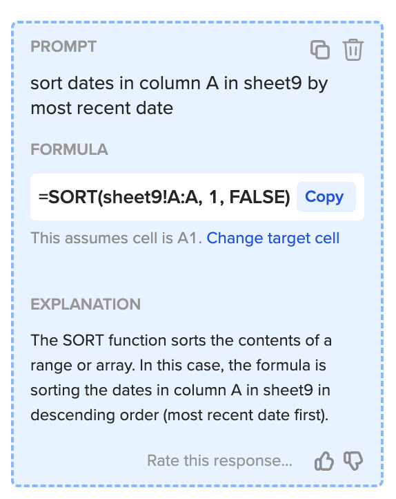
And, it’s that easy! Simply, place the formula in the desired cell.
Unhiding Columns in Google Sheets
Sometimes, you may accidentally hide a column in Google Sheets, or you may have hidden it intentionally but later need to unhide it. Whatever the reason, unhiding columns in Google Sheets is a straightforward process.
Identifying Hidden Columns
Before you can unhide a column, you first need to identify which columns are hidden. You can tell if a column is hidden if you see a double-sided arrow instead of the column letter at the top of the sheet. Alternatively, you can right-click on a cell in the sheet and select “Unhide columns” from the context menu. If the option is grayed out, then there are no hidden columns in the sheet.
Revealing Columns Individually or in Bulk
Once you have identified which columns are hidden, you can unhide them either individually or in bulk. To unhide a single column, click on the double-sided arrow that appears when you hover over the column to reveal a drop-down menu. From there, select “Unhide column” to reveal the column.
If you need to unhide multiple columns at once, you can select all the columns to the left and right of the hidden columns. To do this, click on the column letter of the first visible column to the left of the hidden columns, then drag the mouse to the column letter of the first visible column to the right of the hidden columns. Once you have selected all the columns, right-click on any of the selected columns and choose “Unhide columns” from the context menu.
Managing Columns on Mobile Devices
Google Sheets is also available as a mobile app for both iOS and Android devices. Managing columns on mobile devices is similar to the desktop version, but with a few differences.
Hiding Columns in Google Sheets on iOS
To hide a column in Google Sheets on iOS, follow these steps:
- Open the Google Sheets app on your iOS device.
- Tap the column header of the column you want to hide.
- Tap the three dots in the top right corner of the screen.
- Tap “Hide column” from the dropdown menu.
To unhide a column on iOS, follow these steps:
- Tap the column headers on either side of the hidden column.
- Tap the three dots in the top right corner of the screen.
- Tap “Unhide column” from the dropdown menu.
Hiding Columns in Google Sheets on Android
To hide a column in Google Sheets on Android, follow these steps:
- Open the Google Sheets app on your Android device.
- Tap the column header of the column you want to hide.
- Tap the three dots in the top right corner of the screen.
- Tap “Hide column” from the dropdown menu.
To unhide a column on Android, follow these steps:
- Tap the column headers on either side of the hidden column.
- Tap the three dots in the top right corner of the screen.
- Tap “Unhide column” from the dropdown menu.
