
Google Sheets is a powerful and versatile tool for managing data and organizing information. One often overlooked feature is the ability to compare two columns within a sheet, which can provide valuable insights and streamline data analysis.
Comparing two columns is particularly useful when dealing with large datasets where manual comparisons would be time-consuming and prone to errors.
This article will delve into different methods for comparing two columns in Google Sheets, providing examples and step-by-step instructions.
Comparison of Columns in Google Sheets
In order to compare two columns in Google Sheets, users can employ various built-in formulas and functions. These enable row-by-row comparisons, highlighting exact matches or differences between cell values.
As a result, users can quickly identify patterns, discrepancies, or potential data entry issues, thereby enhancing the overall efficiency and accuracy of data management tasks.
In this section, we will discuss the methods to compare columns in Google Sheets and some common pitfalls and errors you might encounter.
Methods to Compare
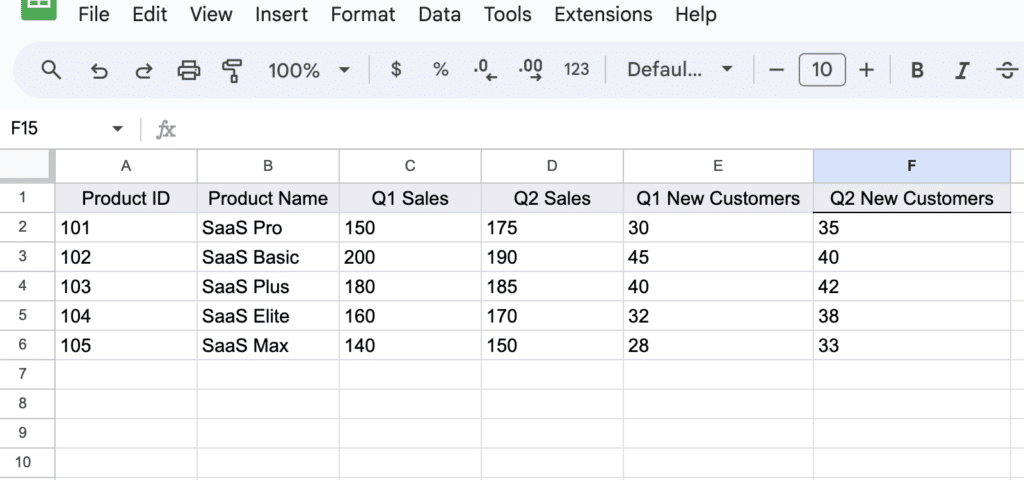
Start by inputting your data into Google Sheets. In this example, we’re working with a simplified dataset representing sales and customer acquisition data for two quarters (Q1 and Q2).
Basic Row-by-Row Comparison for Sales Data
Row-by-row comparison is a fundamental technique in data analysis, allowing for a simple yet effective way to compare values in two columns directly.
This method quickly identifies whether sales figures for a product remain consistent or vary between quarters.
Apply it by inserting ‘=C2=D2‘ in a new column to compare Q1 and Q2 sales.
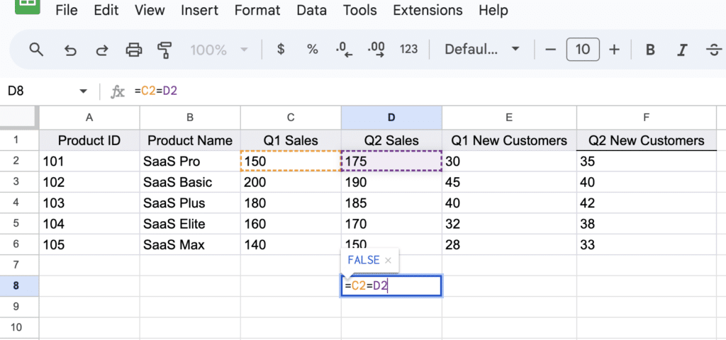
The formula outputs TRUE for equal sales figures and FALSE for any differences, offering a straightforward way to spot sales trends.
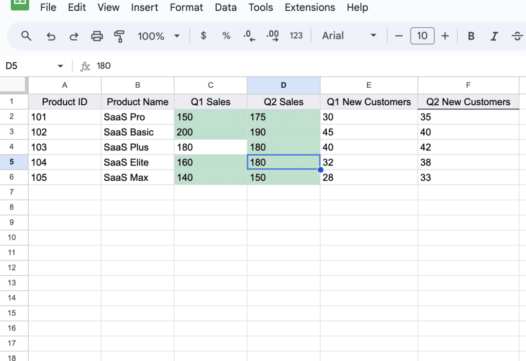
Conditional Formatting to Highlight Sales Variations
Conditional formatting automatically formats cells based on the data they contain, making it easier to visualize patterns and outliers in your data.
This method visually emphasizes products with significant sales changes, allowing for quick identification of major shifts in sales performance.
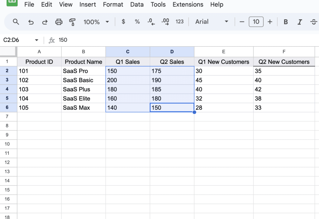
Apply it by selecting the sales data columns (C2:D6).

Supercharge your spreadsheets with GPT-powered AI tools for building formulas, charts, pivots, SQL and more. Simple prompts for automatic generation.

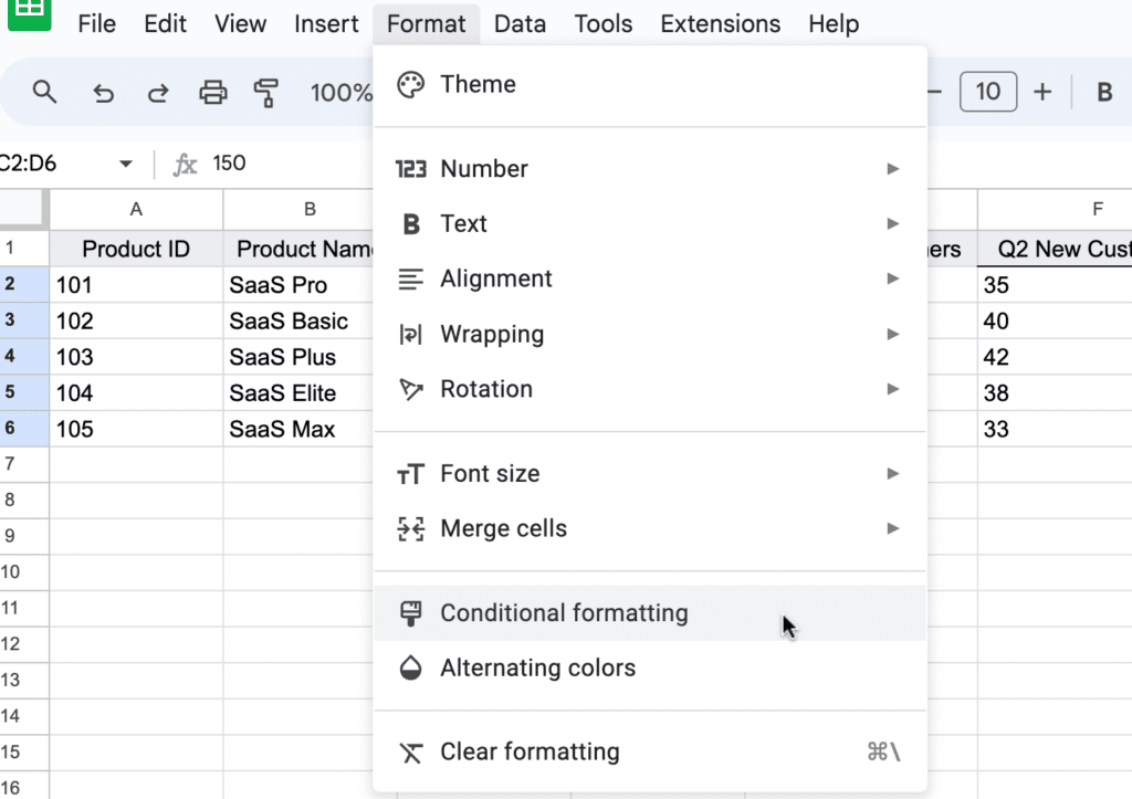
Go to Format > Conditional formatting.
Click + Add another rule.
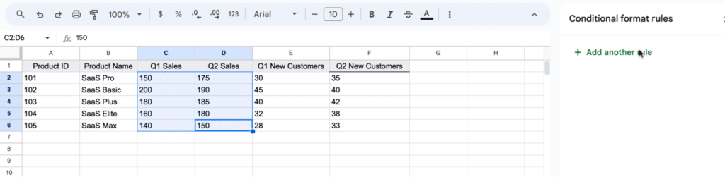
Click the ‘Format rules’ drop-down and scroll down to ‘Custom formula is.’
Enter =C2<>D2 to highlight cells where Q1 and Q2 sales figures differ.
Common Pitfalls and Errors
When comparing columns in Google Sheets, it’s important to be aware of common errors and pitfalls. Some issues you might encounter include:
- Mismatched data types: Ensure that both columns have the same data format. Comparing a column with text values to a column with numerical values might lead to inaccurate results or errors.
- Incorrect formulas: Double-check your formulas to ensure they’re referencing the correct columns and rows. Mistakes in your formulas might yield unexpected results.
- Case sensitivity: Google Sheets comparisons are case-sensitive4. If you’re comparing text data, you may need to use a formula like =LOWER(A2)=LOWER(C2) to ignore the case differences.
Conclusion
By understanding the various methods to compare columns and being aware of the common pitfalls and errors, Google Sheets users can effectively analyze their data and draw meaningful insights from it.
For more advanced data analytics with your business data, consider Coefficient!


