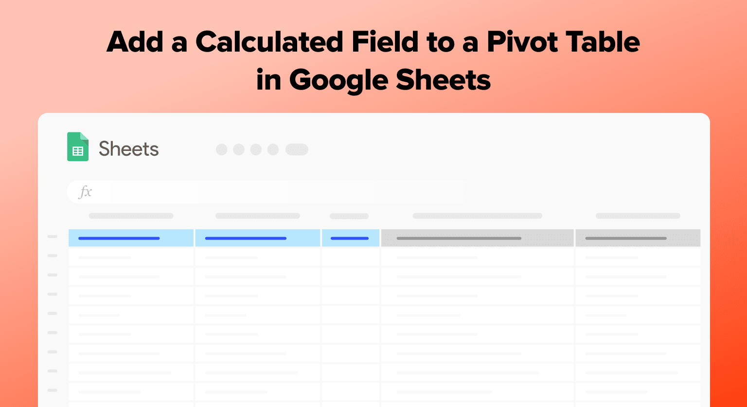

Navigate to the “Data” menu and select “Pivot table” to create your pivot table first
Click the “Add” button next to the “Values” section in the Pivot Table Editor
Select “Calculated Field” from the drop-down menu that appears
Enter your formula in the “Formula” field (e.g., “=sum(price)/count(price)” for average price)
Format your calculated field by clicking “Edit” to change the name or “Format” to adjust number formatting and appearance
Pivot tables in Google Sheets simplify data analysis, but sometimes you need more than the default summaries. Calculated fields are your answer, letting you perform custom calculations directly within your pivot table.
This guide walks you through adding calculated fields to pivot tables, enabling deeper insights without altering your original data.
Creating a Pivot Table
Pivot tables are powerful tools in Google Sheets that allow users to summarize large amounts of data in a flexible and customizable way. To create a pivot table in Google Sheets, users must first have access to Google Sheets and a dataset to work with.
Accessing Google Sheets
Google Sheets is a web-based application that is part of the Google Drive suite of tools. To access Google Sheets, users must have a Google account and be signed in to their account. Once signed in, users can access Google Sheets by navigating to the Google Drive homepage and clicking on the Sheets icon.
Selecting Data for Pivot Table
To create a pivot table, users must have a dataset to work with. The dataset should be organized in a tabular format with rows and columns. Users can select the data they want to use for the pivot table by highlighting the entire dataset or by selecting a specific range of cells.
Inserting a Pivot Table
Once the data has been selected, users can insert a pivot table by navigating to the “Data” menu and selecting “Pivot table.” This will open a new sheet where users can customize their pivot table. Users can drag and drop fields into the “Rows” and “Columns” sections to group and organize their data. They can also add fields to the “Values” section to perform calculations on their data.
In conclusion, creating a pivot table in Google Sheets is a simple process that requires access to Google Sheets, a dataset to work with, and the ability to insert a pivot table. By following these steps, users can quickly and easily summarize large amounts of data in a flexible and customizable way.
Adding a Calculated Field
In Google Sheets, a calculated field is a custom formula that allows you to perform calculations on data in a pivot table. This section will provide a step-by-step guide on how to add a calculated field to a pivot table in Google Sheets.
Opening Pivot Table Editor
To add a calculated field to a pivot table, you need to open the Pivot Table Editor. To do this, click on any cell within the pivot table. Then, click on the “Pivot Table Editor” button that appears in the toolbar at the top of the screen.
Using Formulas for Calculated Fields
Once you have opened the Pivot Table Editor, you can add a calculated field by clicking on the “Add” button next to the “Values” section. This will open a drop-down menu where you can select “Calculated Field.”
In the “Formula” field, you can enter a formula that will calculate the values for your new calculated field. For example, if you want to calculate the average price of products, you can enter the formula “=sum(price)/count(price)”.

Supercharge your spreadsheets with GPT-powered AI tools for building formulas, charts, pivots, SQL and more. Simple prompts for automatic generation.

Formatting Calculated Fields
After you have created your calculated field, you can format it to make it easier to read and understand. You can change the name of the calculated field by clicking on the “Edit” button next to the field name.
You can also change the formatting of the calculated field by clicking on the “Format” button next to the field name. This will allow you to change the number format, font, and other formatting options.
Troubleshooting Common Issues
If you encounter any issues when adding a calculated field to a pivot table, there are a few common problems that you can try to troubleshoot.
One common issue is that the formula is not calculating correctly. Make sure that you have entered the formula correctly and that all of the cell references are correct.
Another common issue is that the calculated field is not showing up in the pivot table. Make sure that you have added the calculated field to the “Values” section of the Pivot Table Editor.
By following these steps, you can easily add a calculated field to a pivot table in Google Sheets.
Conclusion
Adding a calculated field to a pivot table in Google Sheets unlocks custom calculations for more insightful data analysis.
Ready to dive deeper into your data? Coefficient’s AI-powered Pivot Builder allows you to generate Google Sheets pivot tables in seconds with a simple prompt.


