Using the XMATCH Function to Enhance Data Management

The XMATCH function in Excel is a significant tool designed to improve your data lookup abilities. This function permits you to find the position of a precise item within a spectrum or array, offering a more alterable and effective substitute to the conventional MATCH function.

Whether you are functioning with huge sets of data or require accurate matching standards, XMATCH streamlines the process and supports both vertical and horizontal lookups.

In this article, we will traverse how to use the XMATCH function efficiently, indulging its Syntax, Usefulness and Practical Instances to help you get skilled in this helpful Excel function.

What Is The XMATCH Function?

XMATCH is a versatile and powerful function designed to simplify data lookup and retrieval tasks in Excel. This function allows you to search for a specified value within a range of cells and returns the relative position of that value. Unlike the traditional MATCH function, XMATCH offers enhanced functionality and flexibility, enabling you to perform both vertical and horizontal lookups with ease.

With XMATCH, you can search for exact matches, approximate matches, and handle both sorted and unsorted data efficiently. Its ability to conduct lookups in any direction—whether searching across rows or down columns—makes it an indispensable tool for complex data analysis and management.

In this article, we’ll explore deeper into the capabilities of XMATCH, exploring its definition and various use cases. By the end, you’ll have a comprehensive understanding of how to leverage this feature to enhance your Excel projects. Let’s get started!

How Does The Syntax Of XMATCH Work?

The XMATCH function tells you where an item is located in a group of items, like a list or a group of cells in Excel.

=XMATCH(lookup_value, lookup_array, [match_mode], [search_mode])  

Let’s break this down!

The lookup_value is the value you want to find within the lookup_array. It’s what you’re searching for, like a product name or a number. In our example, it would be our data under cell E3, which is “James”

The lookup_array is the range of cells or arrays where you want to search for the lookup_value. It’s like telling Excel where to look, such as a list of products or a column of numbers. In our example, it would be our list of People under C3 to C7.

The [match_mode]  is an optional argument that specifies the type of match you want. If you omit it, XMATCH defaults to an exact match. You can choose from -different match modes like exact match, approximate match, or exact match with wildcards, depending on your needs.

Lastly, the [search_mode] is another optional argument that determines how XMATCH searches for the lookup_value. Again, if you don’t specify it, XMATCH defaults to searching from top to bottom. But you can choose other search modes like searching from bottom to top or searching in sorted order.

Can we see XMATCH in play? Sure thing. Please refer to the below shown image:

Let’s consider a scenario where we have a list of people in cells C3 through C7, and we want to find out the position of the person listed in cell E3 within this list. To achieve this, we will have to utilize XMATCH to identify the item’s location within the list.

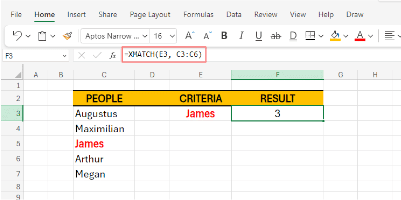
Since James is our selected “criteria” on this example, we can confirm that the yielded result “3” which is equal to “James” is 3rd on our list.

Exploring More About The [match_mode] Option

As mentioned above, the [match_mode] argument determines the type of match you want to perform. Here are the different match types available:

Exact Match (0):

This is the default match type if you don’t specify anything. It returns the position of the first item in the lookup_array that exactly matches the lookup_value. Here is an example:

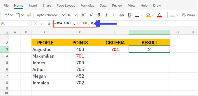
Here we added a new set of points for our participants. Our lookup_value is set to the value of “701”. In our Syntax,

=XMATCH(lookup_value [ E3 ], lookup_array [ D3:D8 ], [match_mode] [ 0 ]).

As a result, our result yielded a value of 2 as our criteria exactly matches the designated point on our table.

Exact Match or Next Largest (1):

This match type returns the position of the closest match that is greater than or equal to the lookup_value. If no exact match is found, it returns the position of the next larger item. Here is an example below:

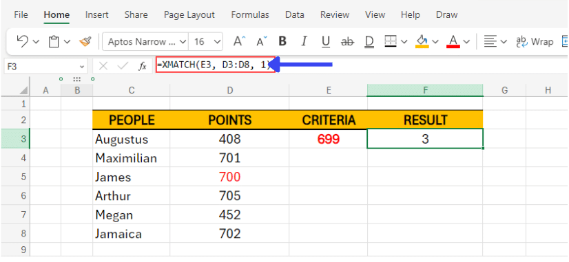
As you can see, our lookup_value has been changed to “699”. For our syntax, we’ve changed the match_mode to (1) which allows our formula to look for the next largest value in our lookup_array, in this case, James with points amounting to 700.

Exact Match or Next Smallest (-1):

Similar to match type (1). This match type is useful when dealing with sorted data. It returns the position of the closest match that is less than or equal to the lookup_value. If no exact match is found, it returns the position of the next smaller item. Here is another example below:

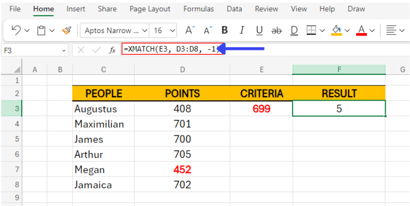
As you’ll be able to see, the yielded value is set to 5 as it matches our list under our table. The syntax selected the cell which had the next lowest value on our lookup_value, which is Megan with a point amounting to “452”.

Wildcard Match (2):

This match type allows you to perform wildcard searches using characters like ‘?’ (matches any single character) and ‘*’ (matches any sequence of characters). It returns the position of the first item that matches the wildcard pattern.

In this example, I’ve changed Jamaica’s point to 408 to demonstrate. I’ve also used the [search_mode] to our syntax to allow our syntax to search our lookup_value from bottom to top. By doing this, our result yielded a value of 6 which is equivalent to Jamaica’s point amounting to “408”

A Quick Run Through Of The [search_mode] Argument In The Xmatch Syntax

The [search_mode] argument in XMATCH function offers flexibility in how you want to conduct your search within the lookup_array. By default (or when set to 1), XMATCH searches from top to bottom of the lookup_array, returning the position of the first matching item found.

Alternatively, setting it to -1 directs XMATCH to search from bottom to top, returning the position of the last matching item found. You can see this example above under the wildcard match we made.

Furthermore, using a [search_mode] of 2 assumes the lookup_array is sorted in ascending order, allowing XMATCH to utilize binary search algorithms for faster performance. In this mode, if an exact match isn’t found, it returns the position of the closest match.

These search modes cater to different scenarios, providing users, such as yourself, with the flexibility to customize their search process based on the nature of your data and specific requirements.

Video Tutorial

Check out the tutorial below for a complete video walkthrough!

Practical Examples Of Using XMATCH

Example #1

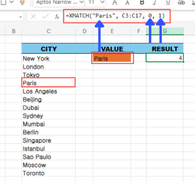
Let’s say we have a list of city names in cells C3: C17, and we want to find the position of a city within a list of cities.

We’ll set our lookup_value to “Paris”.

Explanation:

• “Paris” is the city we want to find.
• C3: C17 is the range where we want to search for the city.
• 0 is the match mode for an exact match.
• 1 is the search mode for searching from bottom to top.

The search mode of 1 indicates that XMATCH should search from bottom to top within the range.

When we enter the formula in a cell, specifically, Cell G4, it will return the position of “Paris” in the list. If “Paris” is in the 4th position from the bottom, the formula will return 4.

This example demonstrates how to use XMATCH with different match modes and search modes to find the position of a city within a list of cities.

Example#2:  Combination Of XMATCH And INDEX Function

What are the basic use-cases of pairing XMATCH with the INDEX function?

Well, let’s first tackle the INDEX function for our better understanding.

The INDEX function in Excel helps you grab specific data from a table or range by indicating the row and column where that data is located. It’s handy for extracting information dynamically, like pulling out sales figures for a particular month or finding a student’s grade from a list.

By specifying the row and column numbers, INDEX allows you to pinpoint exactly what you need from your data, making it a key tool for organizing and analyzing information in Excel.

So how does combining both XMATCH and the INDEX function help me?

XMATCH paired with INDEX functions form a dynamic duo for diverse lookup needs. INDEX complements XMATCH by retrieving corresponding values based on the positions identified, enabling users to extract data efficiently from different ranges. Together, they empower users to perform complex operations like two-way lookups or searches based on multiple criteria, elevating Excel’s data analysis capabilities.

Here is an example:

Let’s say you have an upcoming sales meeting to present the sales of the company for the year. We want to showcase the Item code Ref as they have almost the same first 2 letters under multiple entries.

In this example we used the function of Index to reference our “Item Code Ref” column.

A quick break down on the Syntax we used:

=INDEX(F3:F17,XMATCH(H3&”*”,D3:D17,2,1))

=INDEX(reference[ F3:F17 ], XMATCH(lookup_value [ H3&“*” ], lookup_array [ D3:D17 ], [match_mode] [ 2 ], [search_mode] [ 1 ]).

• The Index reference we used is set to the number of a particular item that the company sold.
• The lookup value is set to cell H3 with a little new twist. We added “&” and “*”. The ampersand and asterisk allows the function to locate items within the lookup value that has the value that we set, in this case, it’s “AH”.
• As for the lookup_array, we’ve set it to D3:D17 for the formula to be able to reference and look for the exact item code in the item code ref column
• As for the match mode, we’ve set it to wildcard, while the search mode is set to 1, this will allow the function to search from top to bottom.

How XMATCH Function Is Useful For Professionals In Marketing, Finance And Data/BI

The XMATCH Function is a significant tool that can be incredibly useful for professionals in marketing, finance and data/business intelligence (BI). Here’s how it can be advantageous each of these fields:

Marketing

1. Customer Segmentation: XMATCH can help marketers segment customers based on numerous norms like buying history, demographics or engagement levels. By locating the spot of precise customers or data points within a list, marketers can easily classify and target them for customized expeditions.
2. Competitor Analysis: Marketers often contrast their products and prices with competitors. XMATCH can be used to find precise competitor information within huge datasets, making it simpler to inspect and collate.
3. Campaign Performance Tracking: XMATCH can rapidly find and cross-reference campaign IDs or metrics within comprehensive data tables, facilitating effective performance inspection when tracking the performance of numerous marketing campaigns.

Finance

1. Portfolio Management: Financial specialists can use XMATCH to rapidly find the location of precise assets or stocks within a collection. This is specifically useful for collection realignment and performance tracking. ‘
2. Budgeting and Forecasting: XMATCH can help in finding precise budget items or financial metrics within huge datasets, assisting in thorough inspection and forecasting.
3. Expense Tracking: Finance teams can use XMATCH to match expenses with their corresponding classifications, ensuring precise expense tracking and reporting.

Data/BI

1. Data Verification: In BI, ensuring data incorporation is crucial. XMATCH can be used to verify data by locating the position of precise entries with a set of data, helping find missing or clone values.
2. Trend Analysis: Data specialists can utilize XMATCH to determine the position of precise time periods or data points within a set of data, expediting trend inspection over time.
3. Report Generation: XMATCH helps in firmly finding and specifying precise data points within large sets of data, making it easier to induce and update reports based on the latest information.

Key Items And Things To Remember In Using XMATCH

Case Insensitivity

In standard use, the XMATCH function in Excel is case-insensitive when searching for text values. This means that it treats uppercase and lowercase letters as equivalent during the search process.

In the above example, since we have a list of cities including “Paris”, upon searching for “paris” using XMATCH, it will still recognize it as a match and return the position of “Paris” within the list.

This case-insensitivity simplifies the search process and ensures that users can find matches regardless of the letter case used in the search query or the data being searched. However, it’s important to note that this behavior applies only to text values and not to numeric or other types of values.

Handling The #N/A? Error

The #N/A? error in XMATCH typically occurs when the specified lookup_value is not found within the lookup_array . This error serves as an indicator that the function couldn’t locate a match for the provided value.

Versatility Of The XMATCH Function

XMATCH is super versatile because it can handle different types of matching in Excel.

• Exact Matching: If you’re looking for an exact match, XMATCH can find it. For example, if you’re searching for “Paris” in a list of cities, XMATCH will locate it exactly where it is.
• Approximate Matching: Sometimes you might not know the exact spelling or value you’re looking for. That’s where approximate matching comes in handy. XMATCH can find the closest match to what you’re looking for, even if it’s not exact. For instance, if you’re searching for “Pris” instead of “Paris,” XMATCH can still find it.
• Partial Matches with Wildcards: Let’s say you want to search for all the fruits that start with “App.” XMATCH can handle that too! You can use wildcards like “?” to represent any single character or “” to represent any sequence of characters. So, searching for “App” would find “Apple,” “Applesauce,” and any other fruit that starts with “App.”

The Benefits of XMATCH for Data-Driven Professionals

XMATCH is an invaluable tool for professionals across various fields. It simplifies data lookup tasks, enabling quick location of specific data points and efficient handling of large datasets. This function enhances accuracy and productivity by streamlining processes such as data validation, trend analysis, and performance tracking. Overall, XMATCH improves the efficiency and effectiveness of data management and analysis, making it an essential tool for any professional dealing with complex data sets.

Using The XMATCH Excel Function

The XMATCH function in Excel offers a powerful tool for efficient data lookup and retrieval, catering to various search scenarios with precision and flexibility. Whether you’re searching for exact matches, approximate matches, or leveraging wildcard patterns, XMATCH streamlines the process, saving time and enhancing accuracy.

With XMATCH, you can efficiently search for exact or approximate matches and handle both sorted and unsorted data. Its capability to perform lookups in any direction—whether across rows or down columns—makes it an indispensable tool for complex data analysis and management.

By comprehending how to use the abilities of the XMATCH function, you can smoothen your productivity and improve the precision of your data handling processes. From simple lookups to intricate array manipulations, XMATCH offers a dependable and effective solution. Practice using XMATCH in numerous outlines to fully relish its advantages and alter the way you manage data in Excel.

If you like the versatility of XMATCH, you’ll love Coefficient, a spreadsheet automation tool to help you to connect to any data source, import live data, automate spreadsheet workflows, and export data into your business systems. Get started with Coefficient today!