Using the SUBTOTAL Excel Function: Real World Examples

Envision you have an enormous set of data in Excel, filled with rows of valuable data. Now you need to perform calculations such as sums, averages and counts but only for precise fragments for your data. As you filter and sort your data, wouldn’t it be marvelous if your calculations optimized automatically to reflect only the noticeable rows? This is where the significant SUBTOTAL function in Excel comes to your ransom.

The SUBTOTAL Function is an adaptable and dynamic tool that permits to perform a variety of calculations on refined or visible data subsets. Unlike standard functions that operate on all rows, SUBTOTAL adjusts to your data view, ensuring your outcomes are always pertinent and up-to-date.

Whether you are handling sales figures, dissecting performance scores, or operating with any large set of data, SUBTOTAL helps you get precise perceptions without the difficulty of continuously optimizing formulas.

In this article, we will discover how to harness the power of the SUBTOTAL function, concealing practical instances and synopsis that substantiates its adaptability and effectiveness.

Performing operations like SUM, AVERAGE, COUNT, MIN, MAX, etc., on a range of cells, the SUBTOTAL Excel function uses specified arguments.

Why Use SUBTOTAL Instead Of SUM?

The benefit of using the SUBTOTAL Excel function (over SUM or any function it performs based on the argument) is that it ignores hidden rows or rows excluded by filters from the calculation. It also ignores cells containing other SUBTOTAL functions when performing any calculation.

So let’s see how exactly the SUBTOTAL function works.

How The SUBTOTAL Excel Function Works

Let’s start with the syntax.

The SUBTOTAL Excel function is defined as: =SUBTOTAL(function_num, ref1, [ref2],…)

For the function_num argument, you’ll need to choose a number for the function you want performed. These numbers are:

function_num	Function	Feature
1	AVERAGE	Ignores only filtered cells
2	COUNT
3	COUNTA
4	MAX
5	MIN
6	PRODUCT
7	STDEV.S
8	STDEV.P
9	SUM
10	VAR.S
11	VAR.P
101	AVERAGE	Ignores both filtered and hidden cells
102	COUNT
103	COUNTA
104	MAX
105	MIN
106	PRODUCT
107	STDEV.S
108	STDEV.P
109	SUM
110	VAR.S
111	VAR.P

As soon as you start typing the SUBTOTAL function syntax, you’ll see all these options in a drop-down menu.

Based on the function_num argument you choose, you can perform the 11 functions listed above. You can also choose the argument to ignore only filtered cells or filtered and hidden cells.

The ref_1 argument is the cell range on which you want to perform the function.

The ref_2, ref_3… ref_255 are optional arguments that contain additional ranges to include in calculating the SUBTOTAL.

Now that you understand how to write a SUBTOTAL Excel function, let’s dive into some examples of how to use it to perform the desired function on a data set.

Examples Of The SUBTOTAL Excel Function

Here are a variety of use-cases for the SUBTOTAL Excel function:

Example #1: Difference Between function_num 1-11 And function_num 101-111

We’ll demonstrate this difference using function_num 9 and 109, both of which will calculate the sum of the given range.

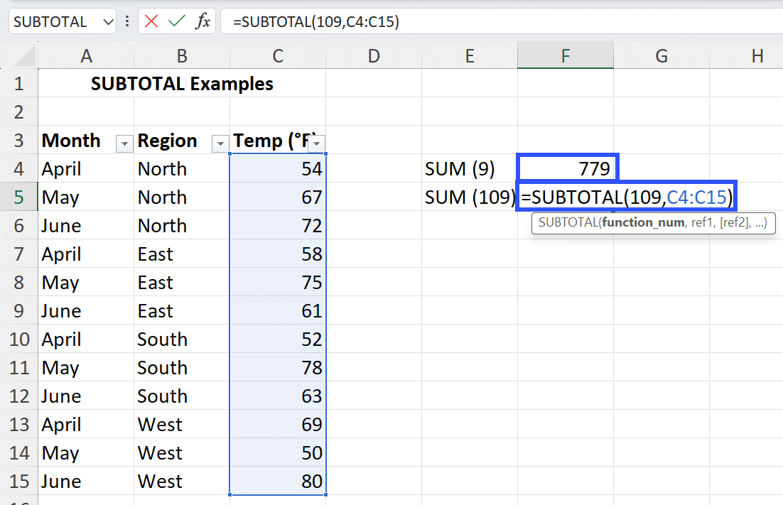
Cell F4 is calculating the SUM using the function_num argument 9, whereas cell F5 is calculating the SUM using the function_num argument 109.

Let’s manually hide rows 12 and 13 and see how the SUM calculation changes:

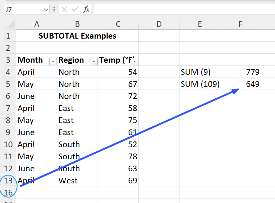
Cell F4 ignores the hidden rows, whereas cell F5 doesn’t.

Now, we’ll filter the table to show all data except the “East” region. Let’s see what impact that has on the two subtotals:

Both the subtotals have ignored the data that has been hidden by the applied filter.

Example #2: Calculating SUBTOTAL Values Of Subsets Within The Main Data Set

If you had to calculate the average/sum/min/max of each region temperature (in the example above), you can use the subtotal Excel function like this:

Now, let’s say you want to calculate the average of all the regions’ temperatures, you can use the SUBTOTAL function across the entire range of temperatures. Like so:

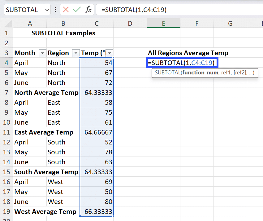
This will return the value 64.91667, which is the average temperature across all regions.

You’ll notice that even though we’ve included each region’s average temperature in the ref1 argument, the SUBTOTAL function in cell E4 ignores those values as they contain separate SUBTOTAL functions.

Example #3: Performing Operations On Data In A Table

The SUBTOTAL Excel function is quite useful when performing operations on data in a table as it ignores cells hidden by a filter.

Let’s say you have a list of products and the respective units sold, and you want to find the highest-selling product for a particular specification. To do so, you’d need to follow these steps:

You’ll identify the maximum value in the “Units Sold” column. But instead of using the MAX function, you’d use the MAX function within SUBTOTAL.

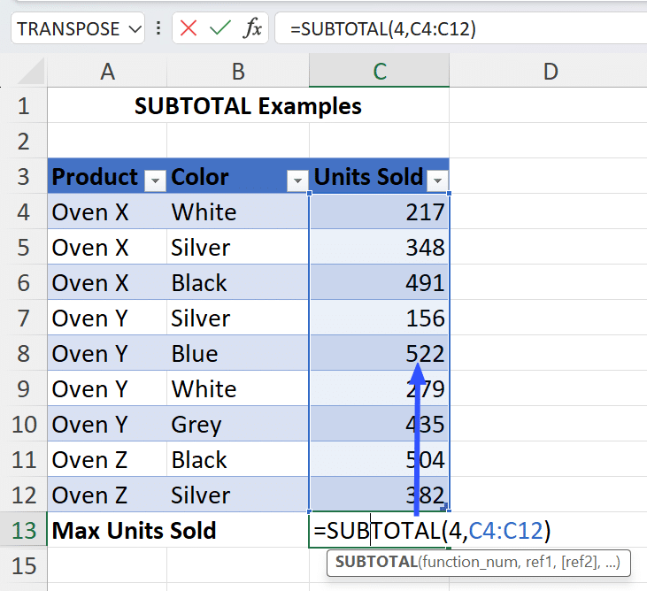
The formula =SUBTOTAL(4,C4:C12) returns the value 522.

Next, you’ll use the INDEX-MATCH function to identify which product this value corresponds to.

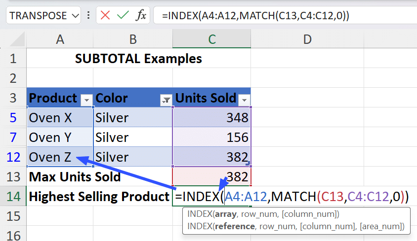
The formula =INDEX(A4:A12,MATCH(C13,C4:C12,0)) returns the value “Oven Y,” which corresponds to 522 units sold.

Now, if you want to identify which is the highest-selling product in “Silver” color, all you have to do is filter the table to show only “Silver” colored products.

You don’t have to even touch any formula to get the data you want, as the SUBTOTAL and INDEX-MATCH functions are already defined in a way to do that for you.

You’ll get the result “Oven Z” in cell C14 as it’s the highest selling “Silver” colored product.

Example #4: Calculating the Average Using SUBTOTAL Function in Excel

Scenario: You have a set of data of employee scores for a department. The set of data indulges the performance score for each employee in a year. You want to calculate the standard performance score while permitting for the adaptability to filter the data and have the standard update spontaneously based on visible rows.

Step-By-Step Instructions:

Launch Excel

Open the excel sheet and enter the data in two rows as shown above.

Enter the SUBTOTAL Formula:

Choose the cell where you want to exhibit the average performance score, for instance cell ‘B12’.

Type the Formula ‘=SUBTOTAL(101, B2:B11).’

As you can see, the average performance score is 85.

Using the ‘SUBTOTAL’ Function with function number ‘101’ permits you to dynamically calculate the average based on the refined data, giving more adaptability in data analysis.

Dealing With Common Errors When Using The SUBTOTAL Excel Function

When using the SUBTOTAL Excel function, you may run into some errors, which can be frustrating. Listed below are the common errors and how to resolve them:

Error Type	Solution
#NAME?	You’ve probably spelled the function name (SUBTOTAL) wrong. Correct the spelling to get rid of this error.
#VALUE!	You’ve entered a value for function_num that is a number not between 1-11 or 101-111. Select the proper value to get rid of this error.
#DIV/0!	You’ll encounter this error when trying to do a mathematical operation on a cell/s that doesn’t contain numerical data. So double check your ref argument.

Now that you’re equipped with knowledge about the SUBTOTAL Excel function, why not take your skills further? Explore how Coefficient can transform your spreadsheet tasks into seamless experiences.

Using The SUBTOTAL Excel Function

This function is an imperative tool for anyone working with huge and dynamic sets of data. Its capability to adjust calculations based on noticeable data, whether refined or sorted, provides a substantial benefit over average functions. With SUBTOTAL, you can smoothly perform numerous operations such as sums, averages and counts, ensuring that your perceptions are always pertinent and precise.

The SUBTOTAL Excel function can help you perform 11 different functions on range, and ignore filtered and/or hidden cells from those calculations.

However, you may not have seen the SUBTOTAL Excel function being used a lot as Pivot Tables offer similar functionality while being more versatile.

Whichever function you choose to use, it will require a good amount of manual data input and repetitive actions. But it doesn’t have to be this way.

With Coefficient, the leading spreadsheet automation tool trusted by over 350,000 professionals worldwide, you can connect to any data source, import live data, and automate spreadsheet workflows. Get started today.