Internal Rate of Return (IRR) calculations are essential for evaluating investment opportunities and making informed financial decisions. In this comprehensive guide, you’ll learn how to use Excel’s IRR function effectively, from basic calculations to advanced scenarios involving multiple investments and irregular cash flows.
How to Calculate IRR in Excel for a Simple Investment
The IRR function in Excel calculates the internal rate of return for a series of cash flows occurring at regular intervals. Let’s start with a basic example.
Step 1: Set Up Your Cash Flow Data
Create a column of cash flows, starting with the initial investment (negative value) followed by expected returns:
|
Time Period |
Cash Flow |
|---|---|
|
0 |
-$10,000 |
|
1 |
$3,000 |
|
2 |
$4,000 |
|
3 |
$5,000 |
|
4 |
$2,000 |
Step 2: Apply the Basic IRR Formula
The basic syntax for IRR is:
=IRR(values,[guess])
Assuming your cash flows are in cells B2:B6, enter:
=IRR(B2:B6)
The result might show 15.32%, indicating the investment yields a 15.32% return.

Using IRR with Irregular Cash Flows
When cash flows occur at irregular intervals, the XIRR function provides more accurate results by considering specific dates.
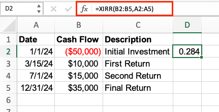
Step 1: Create a Date-Based Cash Flow Table
|
Date |
Cash Flow |
Description |
|---|---|---|
|
1/1/2024 |
-$50,000 |
Initial Investment |
|
3/15/2024 |
$10,000 |
First Return |
|
7/1/2024 |
$15,000 |
Second Return |
|
12/31/2024 |
$35,000 |
Final Return |
Step 2: Apply the XIRR Formula
The XIRR syntax is:
=XIRR(values,dates,[guess])
For the above example:
=XIRR(B2:B5,A2:A5)
Creating an IRR Analysis for Multiple Investments
Compare different investment opportunities by calculating their respective IRRs.
Step 1: Organize Multiple Cash Flow Streams
|
Period |
Investment A |
Investment B |
Investment C |
|---|---|---|---|
|
0 
Try the Free Spreadsheet Extension Over 500,000 Pros Are Raving About
Stop exporting data manually. Sync data from your business systems into Google Sheets or Excel with Coefficient and set it on a refresh schedule. Get Started |
-$20,000 |
-$15,000 |
-$25,000 |
|
1 |
$8,000 |
$5,000 |
$10,000 |
|
2 |
$9,000 |
$7,000 |
$12,000 |
|
3 |
$10,000 |
$8,000 |
$15,000 |
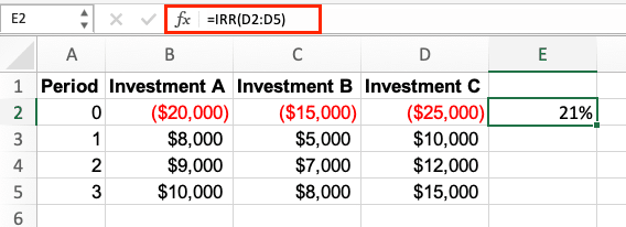
Step 2: Calculate Comparative IRRs
For each investment:
Investment A: =IRR(B2:B5)
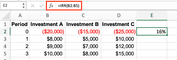
Investment B: =IRR(C2:C5)

Investment C: =IRR(D2:D5)
Handling Complex Investment Scenarios
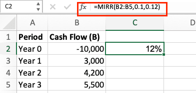
For more sophisticated analysis, use the Modified IRR (MIRR) function, which accounts for different reinvestment and financing rates.
MIRR Formula Example:
=MIRR(values,finance_rate,reinvest_rate)
Practical application:
=MIRR(B2:B5,0.1,0.12)
Where:
- 0.1 represents a 10% financing rate
- 0.12 represents a 12% reinvestment rate
Next Steps
Now that you understand how to implement IRR calculations in Excel, you can enhance your financial analysis by automating data imports and keeping your calculations current. For real-time financial data integration and automated report updates, consider using Coefficient’s Excel add-on.
Get started with Coefficient to streamline your financial analysis workflow and ensure your IRR calculations always use the most current data.


