Introduction To The IFERROR Function in Excel

The IFERROR Function

Tired of dealing with cryptic error messages in your Excel spreadsheets? Meet IFERROR, your go-to solution for managing errors effortlessly. This powerful tool acts as a safety net for your formulas, ensuring that when an error like #DIV/0! or #N/A occurs, IFERROR steps in with a custom message (“Error”) or a blank cell. This keeps your data clean and uninterrupted. Say goodbye to confusing error codes and hello to clear, meaningful results that make your data easier to interpret and work with. Join us below to learn how IFERROR can enhance your Excel experience!

IFERROR Syntax

IFERROR can help you out by checking a formula, and if it evaluates to an error, returns another value you specify; otherwise, returns the result of the formula. Here is the syntax and a breakdown for the Excel IFERROR function:

Syntax: =IFERROR(value, value_if_error)

Value (required): The element to check for errors. This can be a formula, calculation, cell reference, or any other value.

Value_if_error (required): The output displayed when an error occurs. This can be a blank cell, text message, number, or another formula/calculation.

Error Types Handled By IFERROR

The versatility of IFERROR lies in its ability to handle a wide range of error types, making it an essential tool for any Excel user. Here are the common error types that IFERROR can manage:

#DIV/0!: This error occurs when a formula attempts to divide by zero or an empty cell. Using IFERROR, you can replace this error with a more user-friendly message or value.

=IFERROR(A1/B1, “Division Error”)

#N/A: Typically seen in lookup functions like VLOOKUP or HLOOKUP, this error indicates that a value is not available. IFERROR can replace #N/A with a custom message or alternative value.

=IFERROR(VLOOKUP(A1, B1:C10, 2, FALSE), “Not Found”)

#VALUE!: This error arises when a formula encounters an invalid data type. For instance, trying to perform mathematical operations on text. IFERROR can provide a meaningful output instead of the error.

=IFERROR(A1 + B1, “Invalid Data”)

#REF!: This error happens when a reference is invalid, usually due to deleted cells. IFERROR helps maintain clarity by substituting the error with a specified value.

=IFERROR(A1 + B1, “Reference Error”)

#NAME?: This error is due to unrecognized text in a formula, often because of misspelled function names or undefined names. IFERROR can handle this gracefully.

=IFERROR(SUMM(A1:B1), “Function Error”)

#NUM!: This error appears when a formula has invalid numeric values, such as an impossible calculation. IFERROR can intercept and replace it.

=IFERROR(SQRT(-1), “Numeric Error”)

#NULL!: This less common error indicates an incorrect range operator or an intersection of two ranges that do not intersect. IFERROR can simplify handling this error.

=IFERROR(A1 B1, “Null Error”)

When To Use

The IFERROR function in Excel is a powerful tool for handling and managing errors in formulas and data sets, ensuring your spreadsheets remain clean, accurate, and user-friendly. Here’s when you should use IFERROR to enhance your data management:

Handling Division by Zero Errors

Division by zero (#DIV/0!) is a common error in mathematical operations. IFERROR can replace this error with a meaningful message or value, preserving data integrity.

Managing Lookup Failures

Lookup functions like VLOOKUP often return #N/A errors when values aren’t found. Use IFERROR to provide alternative messages or values, making your data more understandable.

Simplifying Data Entry Errors

Errors such as #VALUE!, #REF!, and #NAME? can occur due to incorrect data types or invalid references. IFERROR helps by intercepting these errors and offering clear feedback.

Improving User Experience

Replacing cryptic error messages with user-friendly text enhances the user experience, particularly when sharing spreadsheets with others who may not understand Excel error codes.

Streamlining Data Analysis

In complex analyses, errors can disrupt calculations. IFERROR maintains the flow of analysis by ensuring errors don’t halt your computations.

Ensuring Data Integrity

For multiple error-prone operations, IFERROR ensures final results remain accurate and interpretable.

How To Use And Apply The IFERROR Function

Step 1: Identify the Formula or Expression

To start, identify the formula or expression that you want to evaluate for potential errors. This could be a calculation, a reference to another cell, or any other formula.

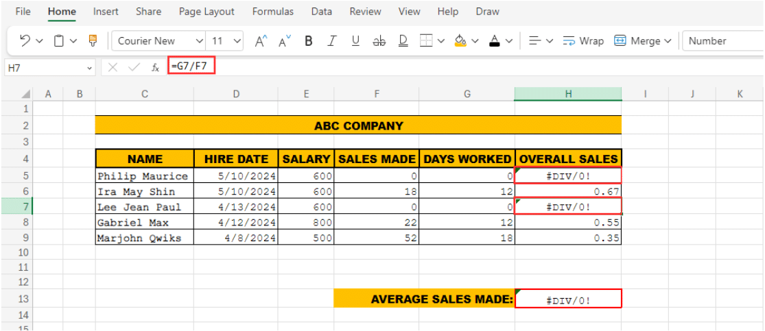
In this example, we want to analyze the overall sales of ABC company. We have determined the company’s data on each salesman hired date, sales record and their total days worked. Under the Overall sales column, we divided their sales made with the total number of days they worked, however, 2 of our employees haven’t started working yet, which renders their sales made and days worked to 0. Here we’ve identified the formula we want to validate for the error message, particularly, cell H3 and H5.

Step 2: Insert IFERROR Function

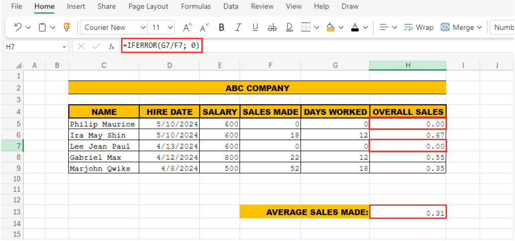
Next, wrap the formula or expression within the IFERROR function. Place the formula you identified as the first argument of the IFERROR function. In this case, we’ve wrapped the formula we had for H3 and H5 with the IFERROR function. A quick breakdown of the syntax:

=IFERROR(value; value_if_error)

=IFERROR(G7/F7; 0)

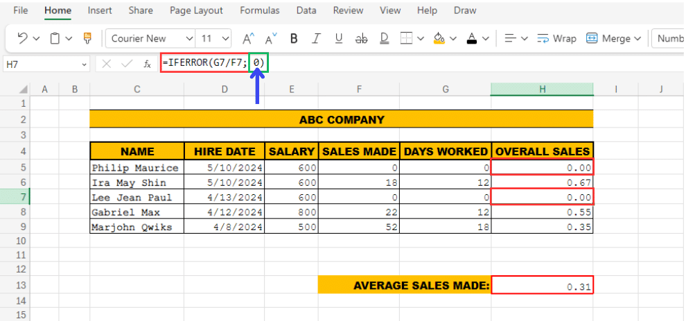
STEP 3: Specify Value if Error Occurs:

Lastly, determine what you want to display if the formula or expression results in an error. This could be a specific value, a text message indicating an error, or another formula. In this example, we used (0) zero to substitute the presented error message for our previous formula.

REMINDER:

• You can also use text for your value_if_error, just remember to place the text under two quotation marks (“ ”). Results may change depending on the data that you’ll be using or applying the formula to.

• You are most welcome to change the zero (0) to better suit your needs. For example, to display nothing, you could use an empty string (“ ”) instead of zero or a text.

Video Tutorial

Check out the tutorial below for a complete video walkthrough!

Practical Examples

IFERROR with VLOOKUP

When using IFERROR with VLOOKUP, you’re essentially creating a safety net around the VLOOKUP function. This combination helps ensure that if the VLOOKUP function encounters an error (such as failing to find a value), your Excel sheet won’t display an error message. Instead, you can specify a custom message or value to display in such cases.

Here is an example, your company has a list of employee IDs in one sheet and you want to look up their names from another sheet. Here we create 2 sheets for this example.

Our Sheet 1 which consist of Employee ID and Employee Name

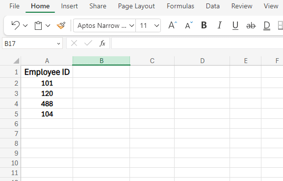
Our Sheet 2 on where we’ll be applying the formula. As you’ll notice, we have 2 different Employee IDs sitting on cell A3 and A4.

Our Syntax:

=IFERROR(VLOOKUP(lookup_value, table_array, col_index_num, [range_lookup]), value_if_error)

Here we applied and filled the formula accordingly. Here’s a breakdown:

VLOOKUP(A2,Sheet1!A2:B2, 2, FALSE): This part of the formula looks up the value in cell A2 of Sheet2 in the range A2:B2 of Sheet1. It tries to find an exact match (FALSE) and returns the corresponding value from the second column (Employee Name).

IFERROR(…, “Not Found”): If VLOOKUP cannot find the value and returns an error (e.g., #N/A), IFERROR catches this error and instead displays “Not Found“.

This use of IFERROR with VLOOKUP helps in handling errors gracefully by providing a user-friendly message instead of a raw error code.

IFERROR In Array formulas

Array formulas can perform multiple calculations on one or more items in an array. When these calculations might result in errors, using IFERROR can help manage those errors gracefully.

Example Scenario 1 

We have two sets of numbers in two columns. We’re going to divide the numbers in the first column by the ones in the second column. If we run into a situation where we’re dividing by zero, instead of showing an error, we’ll display a message we choose or just show zero.

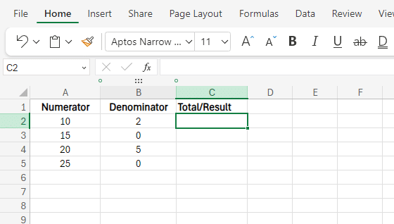
Our aim here is to divide each number in Column A by the matching number in Column B. If the number in Column B is zero, show “Error” instead of #DIV/0!. We have also allotted Column C for the result.

Our Syntax:                                         

=IFERROR(value, value_if_error)

The Formula that you’ll be using:

=IFERROR(A2:A5 / B2:B5, “Error”)

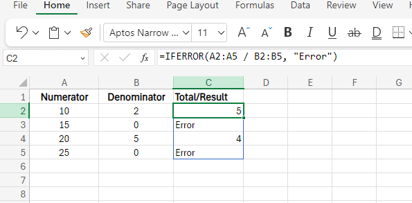
Quick breakdown of the syntax: For the value, we used A1:A4 / B1:B4: This part of the formula attempts to divide each element in the range A1:A4 by the corresponding element in the range B1:B4. While for the value_if_error, we used IFERROR(…, “Error”): If any division results in an error (such as division by zero), IFERROR will catch the error and return “Error” instead. As you’ll be able to deduce, using IFERROR in this array formula helps ensure that any potential errors (like division by zero) are handled smoothly, preventing the display of raw error messages and instead providing a more user-friendly result.

Example Scenario 2

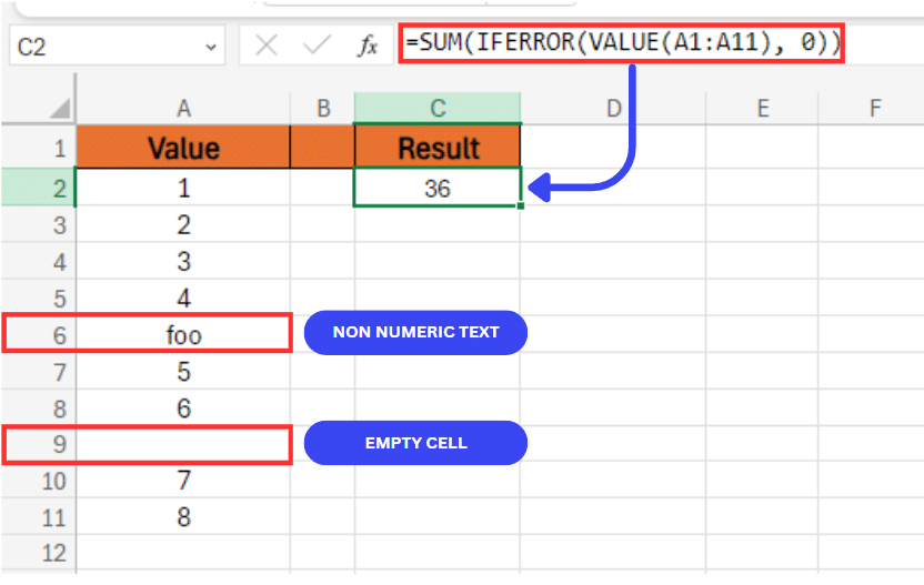
Here, we have a list of values in Column A, some of which are non-numeric (like text or empty cells). We want to convert all the values to numbers and sum them up. Non-numeric values should be ignored and handled gracefully.

Breakdown of the formula:

• VALUE(A1:A11): This part of the formula attempts to convert each element in column A to a number. Non-numeric values will cause an error.
• IFERROR(VALUE(A1:A11), 0): This part of the formula catches any errors from the VALUE function (caused by non-numeric values) and replaces them with 0.
• SUM(IFERROR(VALUE(A1:A6), 0)): The SUM function then adds up all the numeric results, ignoring any non-numeric values that were replaced with 0.

Our second example demonstrates how IFERROR can be used within an array formula to handle non-numeric values during data transformation, ensuring that the final sum calculation is accurate and error-free.

Nested IFERROR For Sequential Lookups

When working with multiple data sources or performing sequential lookups, nested IFERROR functions can be extremely useful. This approach allows you to try multiple lookup operations in sequence and return a result as soon as a successful match is found. If the first lookup fails, IFERROR moves to the next one, and so on, until a valid result is obtained or all options are exhausted.

Example Scenario 1

Let’s say you have data in three different columns, and you want to find a value in the first column that matches your search criteria. If the first column doesn’t have the value, you want to check the second column, and if that fails, check the third column.

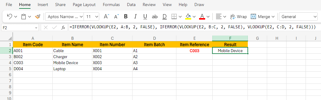
In this example, we have 3 columns that contain the following data for Item Code, Name, Number and Batch. For Cell E1, we have the value that we’re trying to locate.

Here is the breakdown of our formula:

• VLOOKUP(E2, A:B, 2, FALSE): Searches for the value in column A and returns the corresponding value from column B.
• If the first VLOOKUP results in an error (#N/A because the value is not found in column A), the IFERROR function catches the error and proceeds to the next VLOOKUP.
• IFERROR(VLOOKUP(E2, B:C, 2, FALSE): Searches for the value in column B and returns the corresponding value from column C.
• If the second VLOOKUP also fails, the outer IFERROR catches this error and proceeds to the last VLOOKUP.
• VLOOKUP(E2, C:D, 2, FALSE): Searches for the value in column C and returns the corresponding value from column D.

This nested IFERROR structure ensures that the formula will continue to check each column in sequence until a match is found or all options are exhausted.

Example Scenario 2

Suppose you have two tables: Sales and Return tables. You want to find the sales data for a product ID located in cell D10. If the product ID is not found in the Sales table, you want to search for it in the Returns Table. If it’s not found in either table, display “DATA NOT FOUND“.

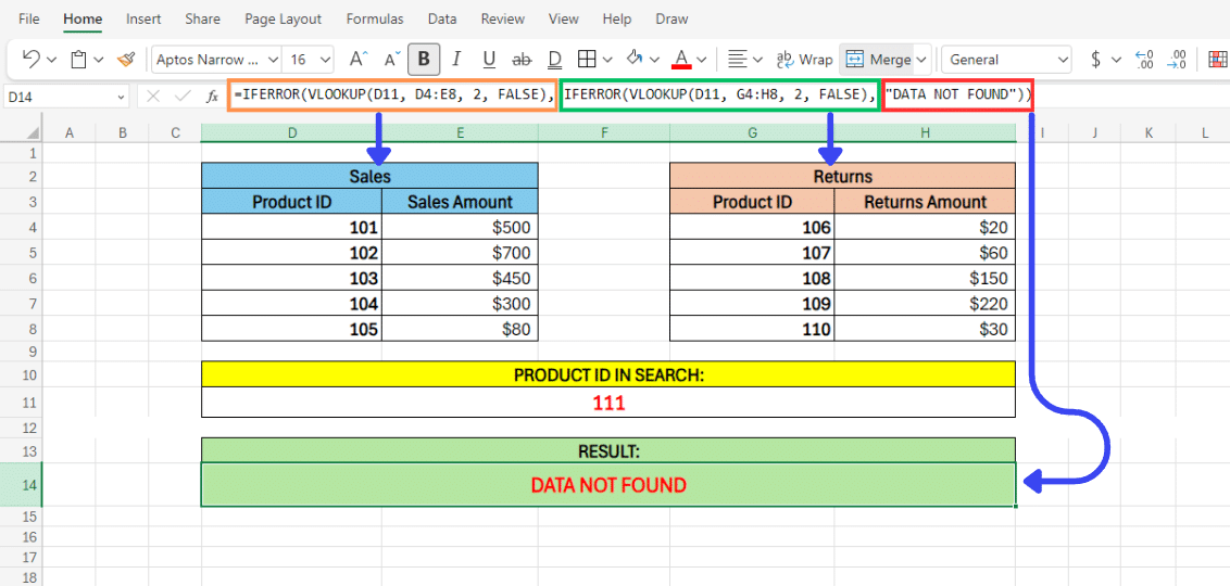
Here is a breakdown of our formula:

=IFERROR (VLOOKUP(D11, D4:E8, 2, FALSE), IFERROR(VLOOKUP(D11, G4:H8, 2, FALSE), “DATA NOT FOUND”))

• The formula first uses VLOOKUP to search for the product ID in the rangeD4:E8 (the Sales table). If the product ID is found, it returns the corresponding sales amount.
• If the product ID is not found in SalesTable, IFERROR catches the error and the second VLOOKUP function searches for the product ID in the range G4:H8 (the Returns table). If the product ID is found, it returns the corresponding return amount.
• If the product ID is not found in either table, the second IFERROR catches the error and the formula displays “Data Not Found”.

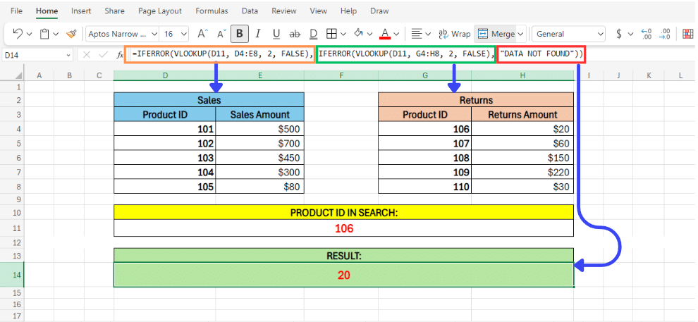
Here you’ll notice that the Product ID in search is set to 106, hence our result yielded the amount it has an equivalent to, which is 20, under our Returns table.

Handling #DIV/0! Errors

The #DIV/0! error in Excel occurs when a formula attempts to divide a number by zero or an empty cell. This can disrupt the readability and functionality of your spreadsheet. The IFERROR function can help manage this error by providing a user-friendly message or an alternative value.

In this example, we’re trying to divide the item’s price with the number of sales. You’ll notice that cell D4 has a missing or empty cell value.

The formula we used divides the value in cell C2 by the value in cell D2. If D2 is zero or empty, the formula returns “Error” instead of displaying the #DIV/0! error. Hence making our data cleaner and easier to understand.

Creating Custom Error Messages Using IFERROR In Excel

The IFERROR function in Excel allows you to replace standard error messages with custom, user-friendly messages. This improves the clarity and usability of your spreadsheets, making them easier to understand and interpret, especially for non-technical users.

In this example, we have a sales data table where we want to look up the sales amount for a specific Item code. We will use the VLOOKUP function to search for the Item code in the table. However, if the Item code is not found in the table, Excel will return the #N/A error. We want to make the error message more user-friendly, you can use the IFERROR function to display a custom message such as “Item code not found”.

If the Item code in E2 is not found in the item sales data table, instead of displaying the #N/A error, Excel will show the custom message “Item code not found”. This makes the spreadsheet more user-friendly and easier to interpret, especially for users who may not be familiar with Excel error codes.

Returning A Blank Instead Of An Error In Excel

In Excel, you can use the IFERROR function to return a blank cell instead of an error message. This is useful for keeping your spreadsheet clean and easy to read.

Here is an example, suppose you are performing a division operation, and you want to avoid showing the #DIV/0! error if the denominator is zero. Instead, you want to return a blank cell.

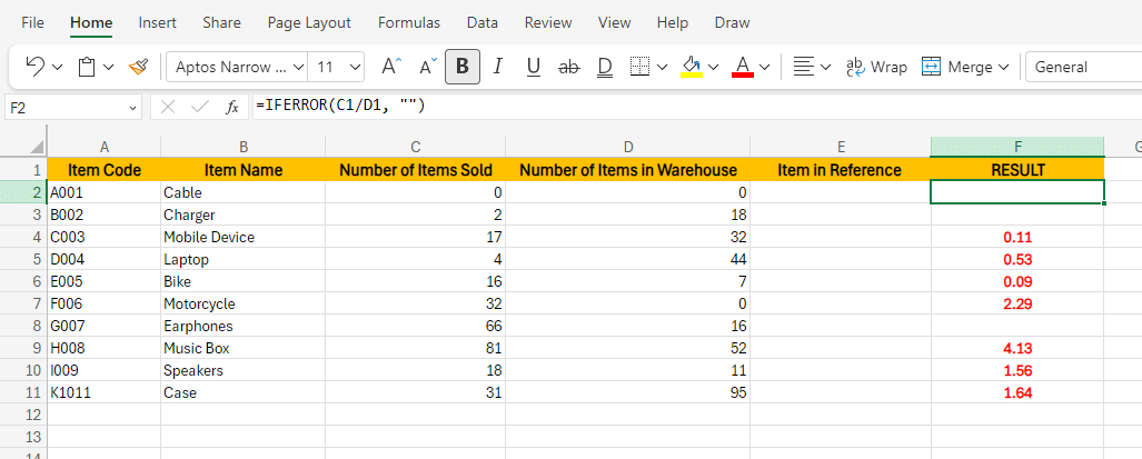
In this above table, since dividing 0, 2, and 66 by 0 would normally result in a #DIV/0! error, the IFERROR function catches this error and returns a blank cell instead.

Comparisons And Best Practices In Excel: IFERROR vs. IF ISERROR, And IFERROR vs. IFNA

In Excel, managing errors effectively is essential for creating clean, user-friendly spreadsheets. Two common methods for error handling are IFERROR and IF ISERROR. Here’s a closer look at their differences and when to use each.

• IFERROR simplifies error handling by combining error checking and handling into one function. This makes it more straightforward and efficient to use.

• IF ISERROR is an older method that requires using the IF function in conjunction with ISERROR. This approach is more verbose and separates error checking from error handling.

• IFNA is for targeted error handling, specifically designed to catch and handle #N/A errors.

Choosing between IFERROR, IFNA, and IF ISERROR depends on the specific needs of your error handling in Excel. We highly recommend properly determining the best use-case for whatever scenario you have. You can use IFERROR for broad error handling, IFNA for handling #N/A errors specifically, and IF ISERROR when you need detailed control over different error types.

Formula Optimization With IFERROR

The IFERROR function in Excel not only handles errors gracefully but also optimizes formulas by simplifying error management. This leads to cleaner, more readable, and more efficient spreadsheets.

Key Benefits:

• Simplified Error Handling: IFERROR allows you to catch and manage errors in a single step. Instead of using multiple IF and ISERROR checks, you can streamline your formula.
• Improved Readability: By using IFERROR, your formulas become shorter and easier to understand. This makes your spreadsheets more maintainable, especially when collaborating with others.
• Enhanced Performance: Simplifying formulas with IFERROR can improve calculation performance. Complex error-checking formulas can slow down large spreadsheets, while IFERROR provides a more efficient solution.

Below, we want to divide numbers in column A by numbers in column B. If the denominator is zero, you want to return a blank instead of the #DIV/0! error.

Standard Approach:

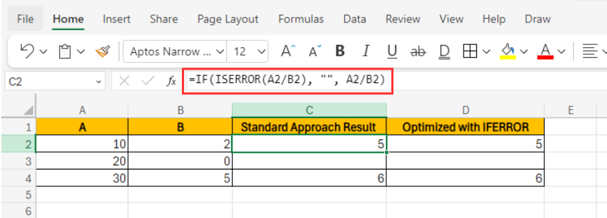
Optimized with IFERROR:

In both the standard approach and the optimized approach using IFERROR, the division by zero in the second row results in a blank cell instead of the #DIV/0! error. The formula using IFERROR is simpler and more concise.

Streamlining Error Handling With IFERROR

In the area of Excel functions, IFERROR stands out as a powerful ally for managing errors seamlessly. Its ability to handle a range of errors, from #N/A to #DIV/0!, simplifies formula construction and enhances the clarity of your spreadsheets.

In this article, we’ve explored the remarkable versatility and efficiency of IFERROR. By integrating error checking and handling into a single function, IFERROR offers a streamlined and elegant alternative to the cumbersome IF and ISERROR combination. This reduces formula complexity and facilitates faster troubleshooting and maintenance.

The simplicity, versatility, and effectiveness of IFERROR make it an essential tool for any Excel user. Whether you’re just starting or are a seasoned pro, mastering IFERROR can greatly improve your spreadsheet productivity and data presentation skills. Embrace IFERROR, and transform the way you work with Excel!

To simplify your tasks, meet Coefficient, the top spreadsheet automation tool. It can link your data sources, automate tasks, and share real-time insights in Excel. Start using it today!