Power Query helps Excel users clean, combine, and update data automatically. Whether you work with sales reports, financial data, or customer lists, Power Query reduces manual work and prevents errors. This guide shows you exactly how to use Power Query, from basic setup to advanced techniques.
Getting Started with Power Query in Excel
Power Query comes built into recent Excel versions. Here’s how to access and set up your workspace:
- Open Excel and select the “Data” tab

- Look for “Get Data” or “Get & Transform Data” in the ribbon

- Click to open Power Query Editor
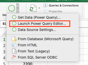
The Power Query Editor has three main sections:
- Query pane (left): Shows your data sources
- Preview pane (center): Displays sample data and changes
- Steps pane (right): Lists all transformations applied
Importing and Transforming Your First Dataset
Let’s start with a basic example using sample sales data.
To import your first dataset:
- Click “Get Data” > “From File” > “Excel Workbook“
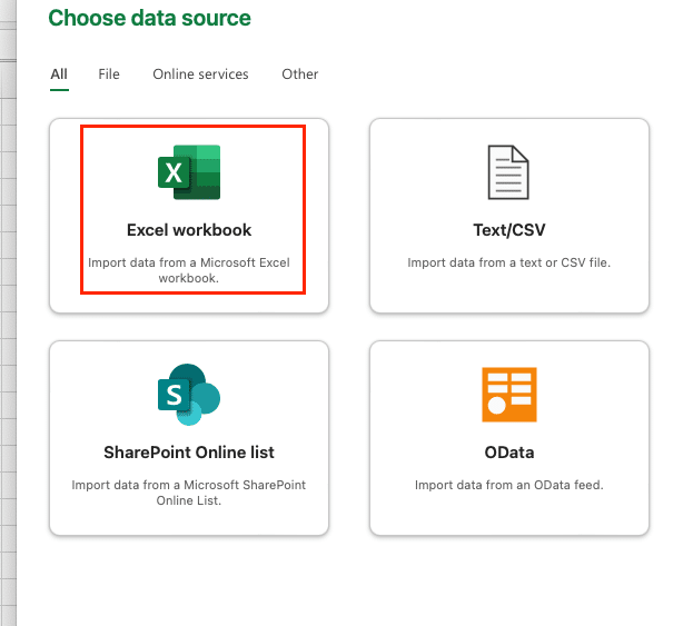
- Select your source file
- Choose the table or range to import
- Click “Transform Data” to open the editor

Pro tip: Start with a small sample of your data while learning. This makes testing faster and easier.
Sample Data Structure
|
Order ID |
Date |
Product |
Quantity |
Price |
|---|---|---|---|---|
|
A101 |
1/1/2024 |
Widgets |
5 |
$10.00 |
|
A102 |
1/1/2024 |
Gadgets |
3 |
$15.00 |
Essential Power Query Transformations
Clean Column Names and Data Types
Follow these steps to standardize your column headers:
- Right-click any column header
- Select “Transform column“

- Choose from options like:
- Remove spaces
- Make uppercase/lowercase
- Remove special characters
To set correct data types:
- Click the icon next to the column name
- Select the appropriate type (Text, Number, Date, etc.)
- Apply to all affected rows
Filter and Sort Data
Create custom filters:
- Click the filter icon on any column
- Choose filter conditions
- Apply multiple filters across columns
Example filter settings:
|
Filter Type |
Column |
Condition |
|---|---|---|
|
Number |
Quantity |
Greater than 10 |
|
Date |
Order Date |
Last 30 days 
Try the Free Spreadsheet Extension Over 500,000 Pros Are Raving About
Stop exporting data manually. Sync data from your business systems into Google Sheets or Excel with Coefficient and set it on a refresh schedule. Get Started |
|
Text |
Product |
Contains “Widget” |
Combine Multiple Data Sources
Merge Tables in Power Query
To combine two related tables:
- Select “Combine > Merge Queries” from the Home tab

- Pick your tables and matching columns

- Choose a join type:

-
- Left outer
- Right outer
- Full outer
- Inner
Append Related Tables
For tables with the same structure:
- Select “Combine > Append Queries” from the Home tab
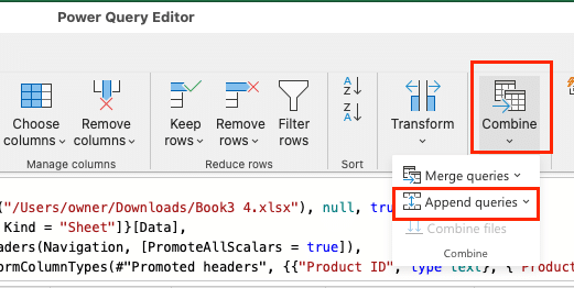
- Choose tables to combine
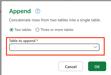
- Review column alignment
- Fix any mismatched columns
Create Custom Columns
Add calculations with these steps:
- Select “Custom Column” from “Add Column” tab
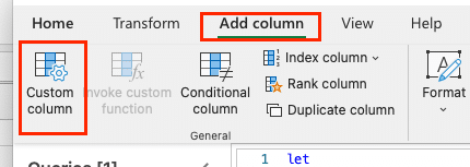
- Enter your formula

- Name the new column
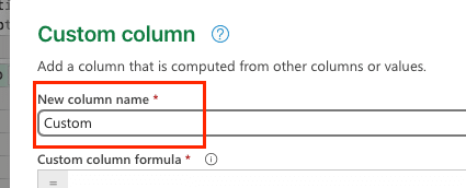
- Click OK
Example formulas:
|
Purpose |
Formula |
|---|---|
|
Total Price |
[Quantity] * [Price] |
|
Full Name |
[First Name] & ” ” & [Last Name] |
Refresh and Manage Queries
Set up automatic updates:
- Right-click query in workbook
- Select “Properties“
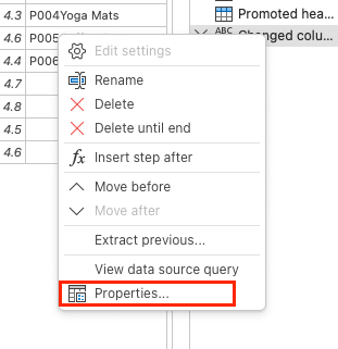
- Choose refresh settings
- Set refresh frequency
Best practices:
- Test queries with small datasets first
- Document your transformation steps
- Keep queries simple and focused
Master Power Query in Excel
Now you can transform Excel data faster and more accurately with Power Query. Start with simple transformations and build up to more complex operations as you gain confidence.
Want to connect your spreadsheets directly to your business systems? Try Coefficient to sync live data from 50+ sources directly into Excel.

