Circular reference errors occur when an Excel formula refers back to its own cell, either directly or through a chain of other formulas. These errors can disrupt calculations and make spreadsheets unreliable. This guide will show you how to identify, fix, and prevent circular references, ensuring your Excel workbooks function correctly.

How to Fix a Circular Reference Error in Excel

When Excel detects a circular reference, it displays a warning message and highlights the problematic cells. Here’s how to address the issue systematically:

Finding the Problem Cells

Step 1: Access the Circular Reference Tracker

1. Navigate to the Formulas tab in the Excel ribbon
2. Look for “Error Checking” in the Formula Auditing group

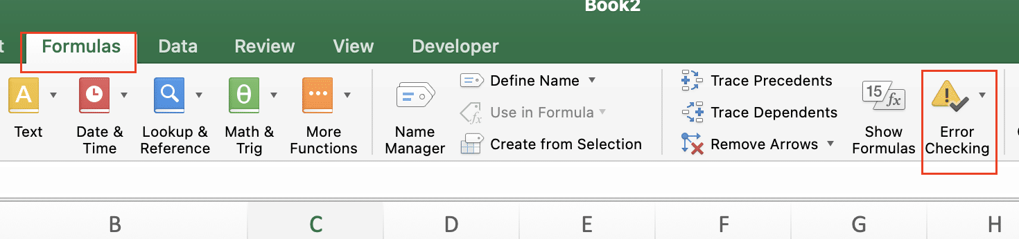
1. Click “Circular References” in the dropdown menu

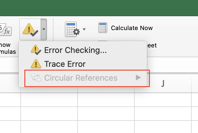
Step 2: Identify Affected Cells

1. Excel will display a list of cells involved in the circular reference
2. Click on each cell to highlight its dependencies
3. Use the trace arrows to visualize the calculation flow

Example of a circular reference chain:

Cell	Formula	Issue
A1	=B1+C1	References B1
B1	=A1*2	References back to A1

Breaking the Circular Reference

Step 1: Analyze the Formula Structure

1. Review each formula in the circular chain
2. Identify which cell calculations can be independent
3. Document the intended calculation flow

Step 2: Reorganize Calculations

1. Start with base values that don’t depend on other cells
2. Build formulas in a logical, one-way sequence
3. Use helper cells to break complex calculations into steps

Example of a corrected structure:

Cell	Original Formula	Corrected Formula
A1	=B1+C1	=C1+D1
B1	=A1*2	=D1*2

Working with Intentional Circular References

Some calculations legitimately require circular references, such as iterative financial models. Excel can handle these through iterative calculations.

Setting Up Iterative Calculations

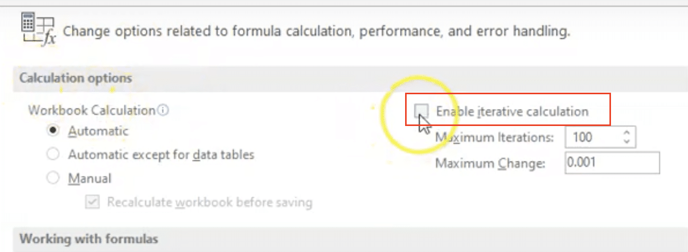
Step 1: Enable Iterative Calculations

1. Go to File > Options > Formulas

1. Check “Enable iterative calculation“

1. Set Maximum Iterations (typically 100)
2. Define Maximum Change (usually 0.001)

Step 2: Configure Calculation Settings

1. Choose between automatic and manual calculation
2. Set iteration limits based on your needs
3. Monitor convergence through the status bar

Formula Restructuring Techniques

Step 1: Implement Helper Cells

1. Break complex calculations into smaller steps
2. Create intermediate calculation cells
3. Document the purpose of each helper cell

Example of helper cell implementation:

Cell	Purpose	Formula
A1	Base Value	100
B1	Helper (10% increase)	=A1 * 1.1
C1	Final Result	=B1 + Other_Calculations

Cell Reference Management

Step 1: Use Absolute References

1. Apply $ signs to lock row/column references
2. Create named ranges for frequently used cells
3. Document reference relationships

Step 2: Establish Clear Dependencies

1. Map calculation flow on paper first
2. Use consistent formula patterns
3. Maintain a one-way calculation flow

Getting it Right

Verify your solution by:

1. Testing with different input values
2. Checking for warning messages
3. Comparing results with manual calculations
4. Documenting your fixes for future reference

Ready to prevent circular references and other Excel errors automatically? Try Coefficient today to catch and prevent formula errors before they impact your work. Get started with Coefficient and ensure your spreadsheets remain error-free.