The GROUPBY function in Excel transforms raw data into actionable insights by creating organized summary views of your information. Whether you’re analyzing sales performance, tracking expenses, or monitoring customer behavior, GROUPBY helps you aggregate and analyze data efficiently.

This guide walks you through everything you need to know about using GROUPBY, from basic summaries to advanced techniques.

Create Your First GROUPBY Summary in Excel

Let’s start with the fundamental process of creating a basic GROUPBY summary.

Step 1: Prepare Your Data

1. Open your Excel spreadsheet
2. Ensure your data has clear column headers
3. Remove any blank rows or columns
4. Format your data as a table (optional but recommended)

Step 2: Select and Group Data

1. Click anywhere within your data range
2. Navigate to Data > Group by (in the Data section)

1. The Group By dialog box appears

Example data structure:

Date	Region	Product	Sales
1/1/2025	North	Widget A	$1,000
1/1/2025	South	Widget B	$1,500

Step 3: Choose Grouping Options

1. Select your primary grouping column (e.g., Region)
2. Choose the values you want to aggregate (e.g., Sales)

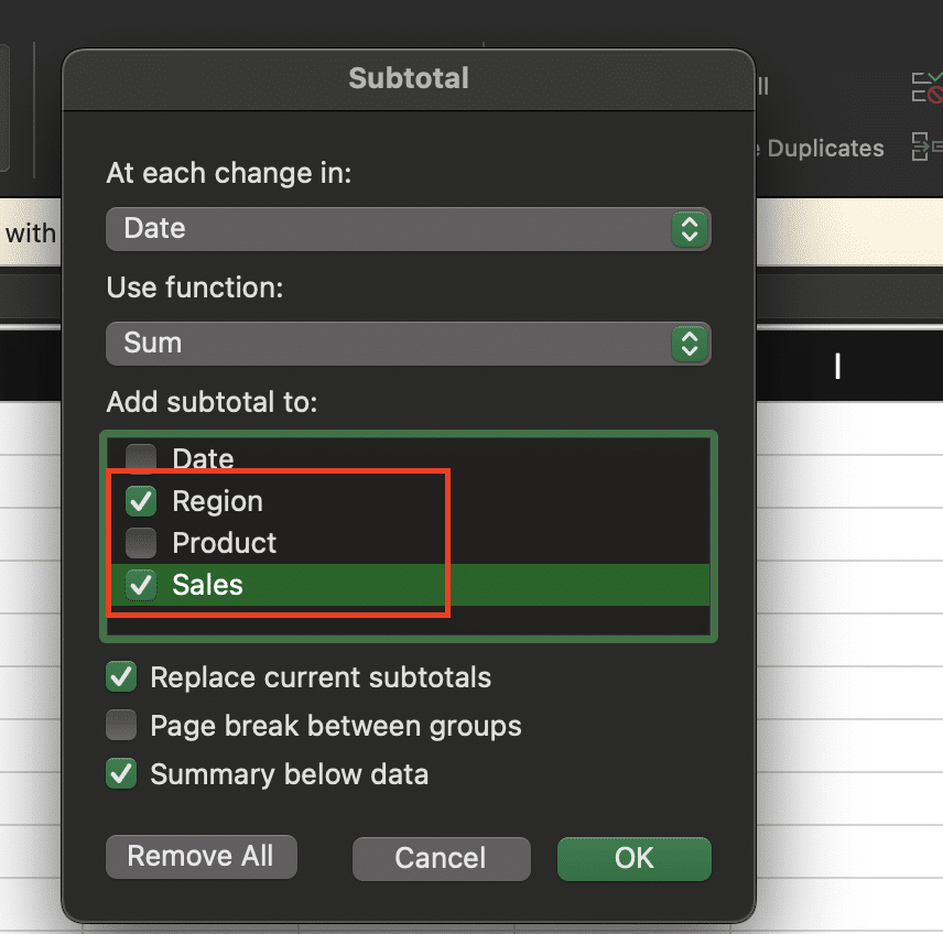
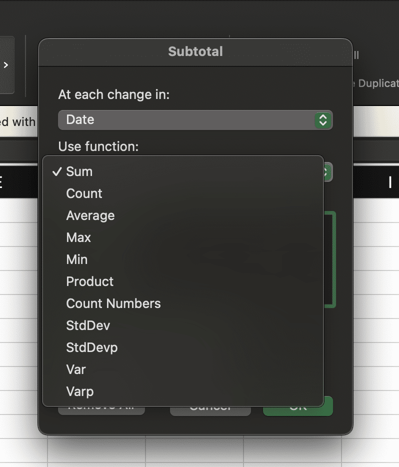
1. Pick your aggregation method:
   • Sum
   • Average
   • Count
   • Min/Max
   • Custom

Step 4: Format Results

1. Apply number formatting to numerical columns
2. Adjust column widths
3. Add borders or shading if needed

Customize GROUPBY Results

Tailoring your GROUPBY output helps create more meaningful and accessible reports.

Step 1: Modify Column Layout

1. Click the “Customize Fields” button
2. Drag columns to reorder them
3. Show/hide specific columns using checkboxes
4. Rename column headers for clarity

Step 2: Adjust Aggregation Settings

1. Right-click on any aggregated column
2. Select “Summarize Values By“
3. Choose from available options:
   • Sum
   • Average
   • Count
   • Min/Max
   • Distinct Count

Example of customized aggregations:

Region	Products Sold	Total Revenue	Avg Order Value
North	Count	Sum	Average
South	Count	Sum	Average

Sort and Filter Grouped Results

Organize your grouped data to highlight the most important insights.

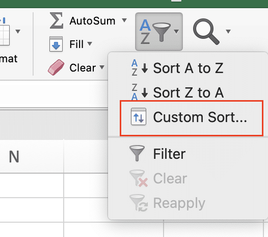
Step 1: Set Custom Sort Orders

1. Select your grouped range
2. Click “Sort & Filter” in the Home tab

1. Choose “Custom Sort“

1. Define multiple sort levels as needed

Step 2: Apply Advanced Filters

1. Click the filter button in your grouped header
2. Select specific filter criteria
3. Use custom filter options for complex conditions
4. Apply date or number ranges

Common GROUPBY Applications

Here are practical scenarios where GROUPBY proves invaluable:

Sales Analysis

• Group by: Region, Product Category
• Metrics: Total Revenue, Units Sold, Profit Margin
• Time periods: Monthly, Quarterly, Annual

Example sales analysis:

Region	Category	Q1 Sales	Q2 Sales	YOY Growth
West	Electronics	$50,000	$55,000	10%
East	Furniture	$45,000	$48,000	6.7%

Expense Tracking

• Group by: Department, Expense Type
• Metrics: Total Spend, Budget Variance
• Time periods: Monthly, YTD

GROUPBY Function Syntax and Options

Understanding the technical aspects helps you create more sophisticated groupings.

Basic Syntax:

 

=GROUPBY(data_range, group_by_col1, [group_by_col2],

[aggregate_function], [aggregate_column])

Available Aggregation Methods:

• SUM: Total values
• AVERAGE: Mean calculation
• COUNT: Number of entries
• MAX/MIN: Highest/lowest values
• COUNTA: Count non-empty cells
• COUNTUNIQUE: Count unique values

Next Steps with Your Grouped Data

Start implementing these GROUPBY techniques today to create powerful data summaries that drive better business decisions. For automated data refreshes and real-time connections to your data sources, try Coefficient’s Excel add-in to streamline your reporting workflow.