Using Excel FILTER Function to Filter Data Dynamically in a Range or Table

FILTER Function In Excel

Do you need help organizing and extracting relevant data from Excel spreadsheets? Introducing the Excel FILTER function, a versatile tool designed to simplify data management.

This function revolutionizes how you handle information by enabling real-time and condition-based data filtering. This guide will explore the FILTER function’s benefits, offering practical examples and advanced tips to enhance your Excel proficiency.

What Does FILTER Function In Excel Mean?

The FILTER function in Excel is convenient to show only the rows that meet your requirements, and the data will be updated automatically as it changes. This function helps to handle information effectively, thus enabling users to narrow down the required data within a short time.

In contrast to the earlier manual filtering and complex formulas typically used, the FILTER function makes the process easier and faster by employing simple syntax and instant results. With this progress, data handling has become more efficient as it is more accessible and reduces data analysis time.

Understanding The FILTER Function

The FILTER function enables Excel users to display data that meet certain conditions, dynamically updating as changes occur within the dataset. The formula of the FILTER function is as follows:

=FILTER(array, include, [if_empty])

Each component of the function plays a crucial role in determining the output. Let’s understand each component in detail:

1. array – This is the range of cells or arrays from which data is filtered. It can be a single column, a row, or a more complex array of multiple rows and columns. The array serves as the source data that you want to refine.
2. include – This is a Boolean array (TRUE or FALSE values) that specifies the conditions under which data from the array will be included in the output. The filtered results will show only the rows or columns that meet the condition(s) expressed in the included parameter.
3. [if_empty] – This is an optional parameter that provides a value to return when no records meet the inclusion criteria. If omitted, the function will return an error if no matches are found. Specifying this parameter helps manage outputs effectively, especially when data may not consistently meet filtering criteria.

To provide a practical demonstration, consider an employee database where you must filter out employees in a specific department earning above a certain threshold. Assume the employee names are in column A, departments are in column B, and salaries are in column C. The FILTER function might look like this:

=FILTER(A2:C100, (B2:B100=”Sales”) * (C2:C100>50000), “No qualifying sales staff”)

In this formula, A2:C100 is the array, B2:B100=”Sales” and C2:C100>50000 are the inclusion criteria (both conditions must be met), and “No qualifying sales staff” is the output if no employees fit those criteria.

Through its dynamic capabilities, the FILTER function significantly enhances data analysis and decision-making processes, allowing for real-time data adjustments and streamlined data presentations in Excel. Let’s understand below in detail.

A Note On Preparing Your Data

To optimize the use of Excel’s FILTER function, it is important to have your data well-organized and structured. Here are some practical tips for preparing your data:

• Uniformity: Ensure that all data in a column is formatted consistently. For example, dates should all follow the same format (DD/MM/YYYY), and text entries should have the same case (all uppercase or all lowercase).
• Completeness: Avoid blank cells in the range or array that will be filtered. Fill in missing data or use placeholder values where necessary to maintain consistency.
• Clarity: Label each column clearly and concisely to reflect the data it contains. This makes it easier to specify criteria in the FILTER function.
• Segmentation: Separate different data types into distinct columns. For example, keep text data separate from numerical values to prevent errors during filtering.

Example of a Well-Organized Table for Dynamic Filtering:

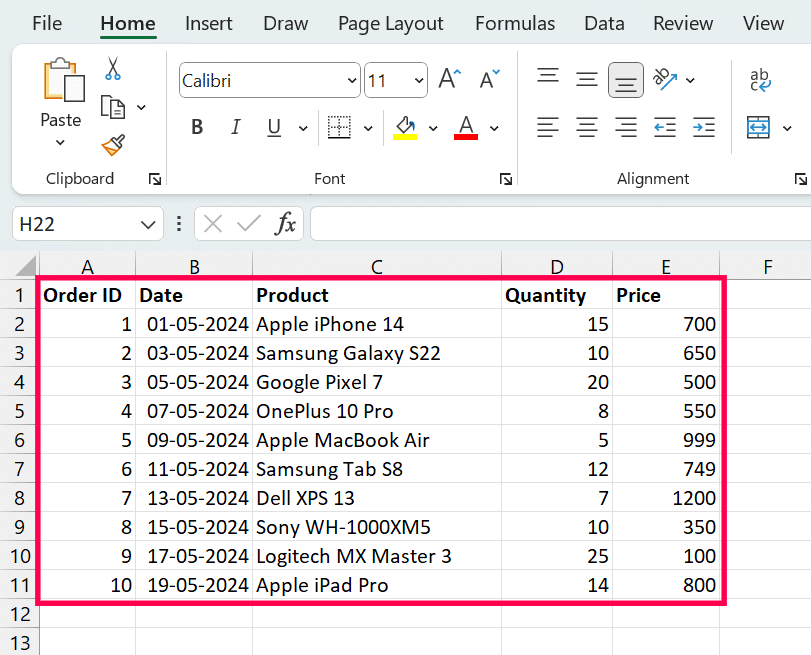
This table is set up for efficient use with the FILTER function, allowing for dynamic filtering based on criteria like product type, quantity, or price.

Video Tutorial

Check out the tutorial below for a complete video walkthrough!

Examples Of The FILTER Function

The FILTER function in Excel is powerful for displaying data based on specified conditions. The simplicity or complexity of these conditions can range from a single criterion to multiple criteria, affecting the function’s versatility.

One Criterion involves filtering data based on a single condition, such as displaying all products with a price above $500. Multiple Criteria include combining two or more conditions, possibly across different columns, like displaying products with a price above $500 and a quantity below 15.

Example 1: Filter Data Based on One Criterion

Here’s a step-by-step guide on how to use the FILTER function with one Criterion using the well-organized table provided:

Step 1: Select the Cell for Results

Choose the cell where you want the filtered results to display. For example, select cell G2.

Step 2: Enter the FILTER Function and Define the Range for the Array

The range of the data table is A2:E11, which includes all the data rows from the ‘Order ID’ to ‘Price’ columns. In your formula bar, it would look like this “=FILTER(A2:E11,“

Step 3: Set the Condition for Include

The condition set for inclusion is D2:D11 > 10, which filters the data to show only those rows where the quantity is more than 10. The formula would be “=FILTER(A2:E11, D2:D11 > 10“.

Step 4: Close the Formula and Press Enter

Press Enter after typing the formula. The rows meeting the Criterion will appear starting from cell G2.

In this case, we want to filter out all products with a quantity greater than 10.Syntax:

=FILTER(A2:E11, D2:D11 > 10)

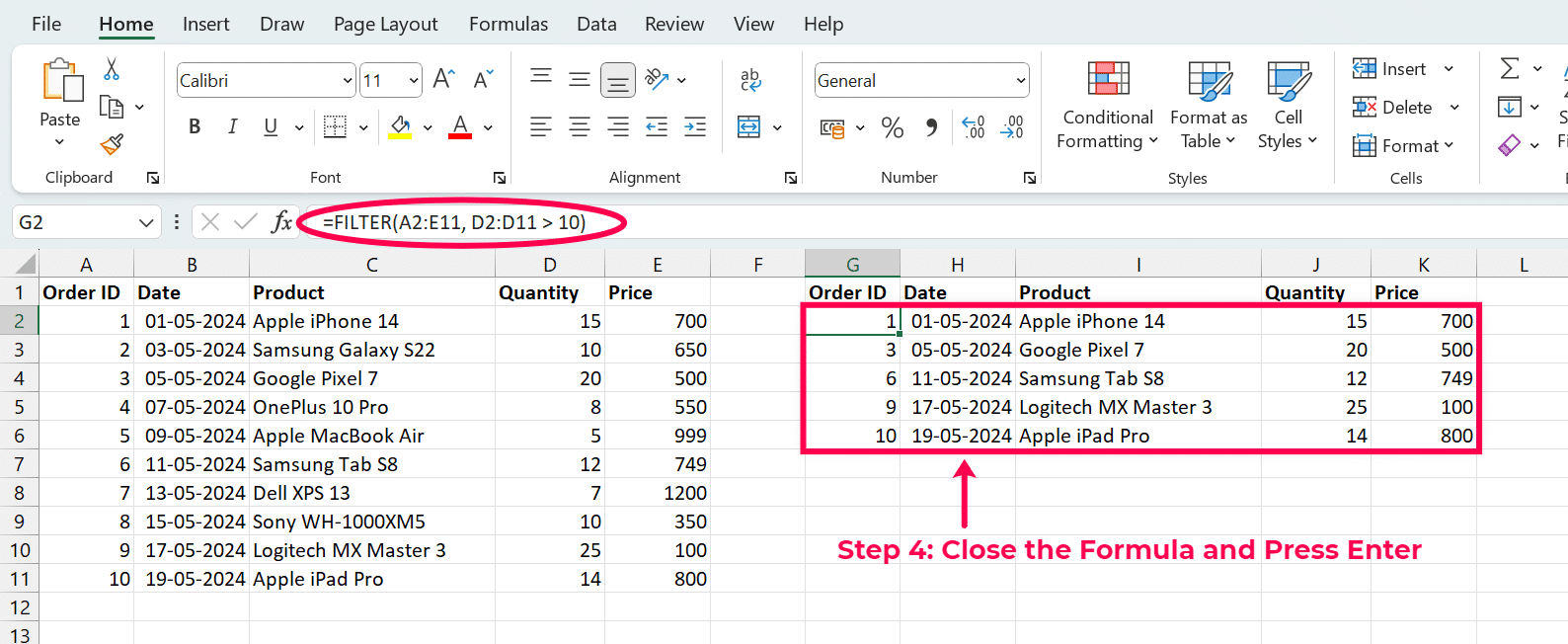
The filtered results will include all entries with quantities greater than 10. Depending on the actual data, this might consist of rows for Apple iphone 14, Google Pixel 7, Samsung Tab S8, Logitech MX Master 3, and Apple iPad Pro, among others.

Example 2: Filter Data Based On Multiple Criteria

To effectively filter data using multiple criteria in Excel, follow these detailed steps using the FILTER function. This example will use the dataset provided, which includes various electronic products.

Step 1: Select the Cell for Results

Click on an empty cell where you want the filtered results to appear. I added “G2” to the data table to avoid overwriting existing data.

Step 2: Enter the FILTER Function with Multiple Conditions

Type the FILTER function into the selected cell. Suppose you filter the data to show only items with a price greater than $500 and a quantity less than 15. The formula will look like this: “=FILTER(A2:E11, (E2:E11 > 500) * (D2:D11 < 15))“

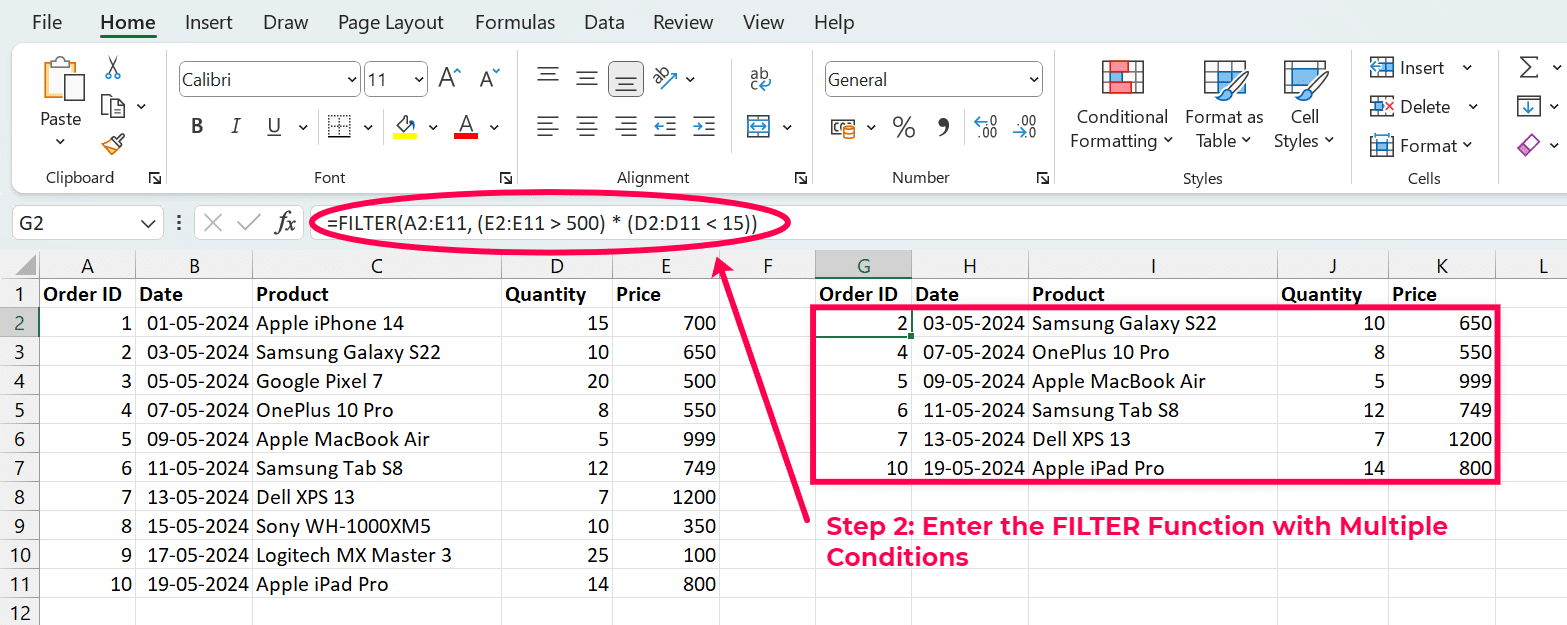
Here’s what each part of the formula represents:

• ‘A2:E11‘ is the range of your dataset.
• ‘E2:E11 > 500‘ is the condition that the price must exceed $500.
• ‘D2:D11 < 15‘ is the condition that the quantity must be less than 15.
• ‘*‘ is a multiplication sign used as an AND operator to ensure that both conditions must be valid for the data to be included in the filter.

After entering the formula, press Enter. Excel will dynamically display the filtered data based on the specified criteria in the cell where you entered the formula. For our example with AND conditions, Excel filters and shows the rows that meet both conditions (price > $500 and quantity < 15).

Step 3: Learn How to Use Logical Operators (AND, OR) Within the Function

AND Operator (‘*’): Use the FILTER function’s multiplication symbol (‘*’) as the AND operator. This means that all conditions separated by ‘*’ must be valid for a row to be included in the results.

OR Operator (‘+’): Alternatively, you can use the addition symbol (‘+’) as the OR operator. If any conditions are proper, the results will include the row. For instance, to find products either priced over $1000 or having less than 10 items in quantity, the formula would be “=FILTER(A2:E11, (E2:E11 > 1000) + (D2:D11 < 10))”

By following these steps, you can filter your data dynamically using multiple criteria in Excel. This method allows for versatile data analysis and can adapt to various scenarios by changing the requirements.

Advanced Usage Of The FILTER Function

Expanding your proficiency with the FILTER function in Excel can significantly enhance your data analysis capabilities. Below are some advanced techniques to make the most out of this powerful function:

1. Use Wildcard Characters for Partial Text Matches:

Excel’s FILTER function can incorporate wildcard characters, such as ‘*’ (asterisk) and ‘?’ (question mark), to perform partial text matches. The asterisk ‘*’ represents any sequence of characters, and the question mark ‘?’ stands for any single character.

For Example: To filter a list of products to find any that include the word “Phone,” use the formula: “=FILTER(A2:B10, ISNUMBER(SEARCH(“*Phone*,” B2:B10)))”. This formula checks the range B2:B10 for any occurrence of “Phone.”

1. Handling Errors and Empty Outputs with the [if_empty] Argument:

The ‘[if_empty]’ parameter in the FILTER function specifies what to display when no elements meet the set criteria. It is beneficial for maintaining the cleanliness and usability of your data output by avoiding #CALC! Errors when the result is empty.

For Example, if you want to display “No Matches Found” when no results match the filter criteria, use “=FILTER(A2:B10, B2:B10=”Specific Criteria”, “No Matches Found”).”

1. Combining FILTER with Other Functions (e.g., SORT, UNIQUE):

FILTER can combine with other functions to provide more complex and dynamic analyses.

Sorting Filtered Data: Combine FILTER with SORT to organize the filtered output. Example: ‘=SORT(FILTER(A2:B10, B2:B10=”Active”))’ will filter for “Active” entries and then sort these entries in ascending order.

Removing Duplicates from Filtered Data: Use FILTER with UNIQUE to eliminate duplicates from the results. Example: =UNIQUE(FILTER(A2:B10, B2:B10=”Active”)) filters for “Active” statuses and removes any duplicate entries from the filtered list.

These combinations are powerful for creating dynamic reports that update and refine data based on your specified conditions.

Here are two additional examples that can further enhance your data analysis skills:

1. Filter Based on Multiple Conditions:

To filter this dataset for active status and sales above 50, use the formula “=FILTER(A2:D11, (B2:B11=”Active”)*(D2:D11>50))”

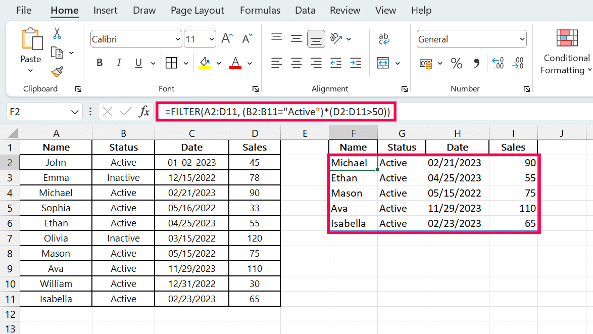
This will result in a filtered dataset showing only the active names with sales greater than 50.

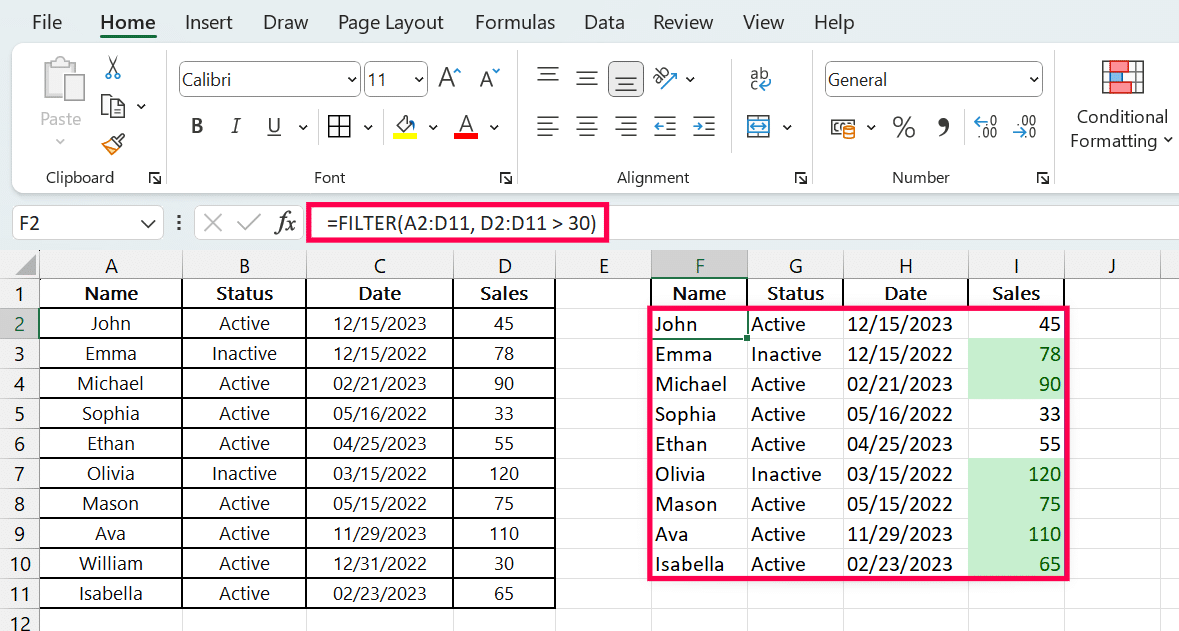
2. Conditional Formatting of Filtered Results:

After applying the FILTER function to get all products with sales over 30, apply conditional formatting to highlight products with sales over 60. First, apply the filter “=FILTER(A2:D11, D2:D11 > 30)”.

Then select the resulting cells in the “Sales” column and use Excel’s conditional formatting tool to set a rule that fills cells greater than 60 with a specific color.

These advanced techniques allow you to manipulate and analyze your data in Excel more effectively, making the FILTER function a versatile tool for complex data tasks.

Dynamic Filtering With Real-Time Data

Real-time data management is crucial for making informed decisions in today’s fast-paced environment. By integrating Excel’s FILTER function with Coefficient, professionals can achieve dynamic filtering with automatic updates, ensuring data remains current and actionable. Coefficient streamlines connecting Excel Tables to various data sources like Salesforce, HubSpot, and SQL databases.

This integration allows the FILTER function to apply criteria dynamically to live data feeds directly within Excel. As a result, tables update automatically as source data changes, eliminating the need for manual refreshes and data re-entry.

For example, when using Coefficient with external databases, you can set up dynamic filters that adjust based on real-time market trends or customer behavior insights. This capability ensures that your Excel datasets always reflect the latest information, providing a solid foundation for strategic planning and analysis.

Moreover, Coefficient’s robust data filtering options enhance the functionality of the FILTER function by allowing users to specify complex criteria and conditions for data retrieval. This integration saves time and increases the accuracy and relevance of data analyses.

To experience seamless real-time data integration and dynamic filtering in Excel, start your free trial with Coefficient today to see how it can transform your data management strategy. This tool is essential for anyone looking to elevate their use of Excel with live, actionable insights.

Common Problems With The Excel FILTER Function And Their Solutions

1. Error: #CALC!

This error occurs when the FILTER function attempts to return a large array that exceeds the worksheet’s row or column limits. To resolve, limit the range of the data or split the function into multiple smaller arrays.

2. Error: #VALUE!

Incorrect data types within the arguments can cause conflicts. Ensure that the ‘include’ argument is a Boolean array and that the ‘array’ consists of compatible data types.

3. Error: #SPILL!

This error is caused by insufficient space around the output area, which can block the function’s ability to display results. The solution is to clear adjacent cells to the formula to provide enough space for the array to spill.

4. Performance Lag with Large Datasets

The FILTER function becomes slow or unresponsive when handling large datasets. Excel tables, which are optimized for performance and can dynamically manage ranges, are used to manage the data efficiently.

5. Error: Array size mismatch

Cause: The size of the ‘include’ array does not match the size of the ‘array.’ The solution is to ensure the ‘include’ Boolean array matches the dimensions of the ‘array’ being filtered.

Optimizing FILTER Performance

Pro Tips: Avoid volatile functions as criteria within the FILTER function to prevent excessive recalculations. Utilize Excel’s Data Model feature to handle large datasets effectively. This reduces the in-sheet data footprint by linking directly to external databases. Apply filters to the smallest possible data range to reduce computation overhead. When using the FILTER function, it is recommended to use defined names for ranges to improve the readability and work with the formulas. It is easier to debug and modify defined names than when using cell references, especially when working with multiple FILTER functions.

Real-World Applications

• Business Inventory Management: The FILTER function dynamically tracks inventory levels across multiple warehouses. Managers can instantly see which items need restocking, optimizing the supply chain. (Learn more about inventory management techniques).
• Educational Data Analysis: Teachers can filter student performance data to identify trends and areas for improvement. It allows for targeted interventions and personalized learning plans, boosting educational outcomes.
• Personal Finance Tracking: Individuals can use FILTER to manage their budgets by categorizing expenses and automatically updating spending summaries. This helps maintain financial discipline and achieve savings goals more effectively.
• Sales Reporting: Sales teams can generate real-time reports showing sales by region, product, or team. Dynamic filtering accelerates the decision-making process and enhances responsiveness to market changes.
• Customer Service Analysis: Filter customer feedback by issue type, urgency, or satisfaction level to prioritize responses and improve service quality efficiently.

These applications demonstrate how the FILTER function can dramatically enhance efficiency and productivity in various real-life contexts.

Ready to streamline your data management? Try Coefficient today for seamless data integration, automated workflows, and real-time insights. Get started now!