
Introduction To The Excel SORT Function
The Excel SORT function can sort your data in ascending or descending order, whether you are dealing with numericals, dates or text.
Since SORT belongs to the group of dynamic array functions that automatically spills to neighboring cells, it is useful when operating with large datasets, eliminating the need for manually updating the array each time.
There is another function that can help you organize data–SORTBY. Let’s see how they compare.
SORT vs. SORTBY: A Simpler Alternative
SORT offers a direct technique where you can simply rearrange data based on the values in any one column. Comparatively, SORTBY provides advanced sorting options for more intricate scenarios.
The obvious benefit is that it’s far easier to understand and use SORT (compared to SORTBY). So let’s start with understanding the syntax.
Excel SORT Function Syntax
The common Syntax for the Excel SORT Function is =SORT(array, [sort_index], [sort_order], [by_col])
Let’s look at each argument in function:
- array: This defines the array that you want to sort. It can be a solitary column, a row, or a multi-column array.
- sort_index: This argument defines the row or column index of the array that you want to sort by. The default value is 1, which means it will sort by the first row or column.
- sort_order: This is an optional argument that defines what order to sort the array in. Setting it as 1 sorts in ascending order (default), while -1 sorts in descending order.
- by_col: This is also an optional argument that defines whether the sort should be done by column or by row. Setting it to TRUE sorts by column, whereas setting it to FALSE (default), sorts by row.
Next, let’s look at some simple examples of how to use the Excel SORT function, to clarify what we just discussed.
Using The Excel SORT Function
Here are some simple ways to use the Excel SORT function.
Example #1: Basic Sort
You can use the default settings of the Excel SORT function by using the formula: =SORT(A4:D15)

This function returns the whole array, sorted in ascending order of values in the first column of the array (i.e., Name).
Example #2: Sorting By Different Columns
If you wanted to sort the array by the values of a different column, say Result column, you can define the sort_index argument in the formula accordingly: =SORT(A4:D15,4)

This function returns the whole array, sorted in ascending order of values in the fourth column of the array (i.e., Result).
Example #3: Sorting In A Different Order
Now, if you wanted to sort the array by Result, but from the highest to lowest score, you can define the sort_order argument as -1. Thus, the formula becomes: =SORT(A4:D15,4,-1)
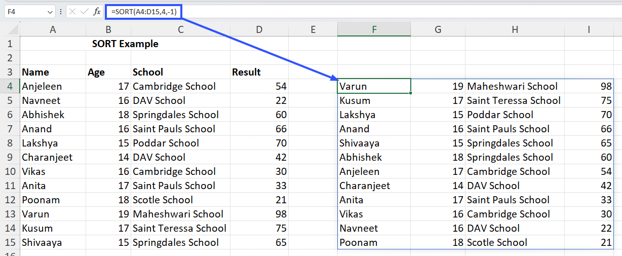
This function returns the whole array, sorted in descending order of values in the fourth column of the array (i.e., Result).
Example #4: Sorting Data In Columns (Instead Of Rows)
If your data was in a columnar format (instead of in rows), you can set the by_col argument to TRUE to sort columns instead of rows. The formula becomes: =SORT(B4:M5,2,1,TRUE)
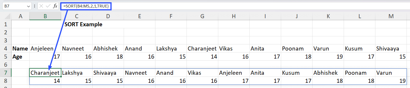
This function returns the whole array, sorted in ascending order of values in the first row of the array (i.e., Name).
Example #5: Sorting Multiple Columns In A Different Order (Multi-Level Sort)
When sorting a list of student names by age, there could be multiple students of the same age. So you’d want to sort students of the same age in ascending alphabetical order of names.
The formula you’d use for that is: =SORT(A4:D15,{2,1})

This function returns the whole array, sorted in ascending order of values in the second column (i.e., Age). And when the Age is the same, it sorts those values in ascending order values in the first column (i.e., Name).
Now, if you want to sort in descending order of age and names, you’d define the both sort_index and sort_order in arrays like this: =SORT(A4:D15,{2,1},{-1,-1})

This function returns the whole array, sorted in descending order of values in the second column (i.e., Age). And when the Age is the same, it sorts those values in descending order values in the first column (i.e., Name).
These are just a few ways to sort data using the Excel SORT function, but text and numbers are not the only way to sort data.
Different Ways Of Sorting Data In Excel
We have already shown how to sort data in Excel using text or numbers. Given below are the other ways of sorting data in Excel:
Sorting By Dates
Since Excel treats dates as numbers, you can sort a range based on date values by using the basic SORT formula: =SORT(A5:C16,3)
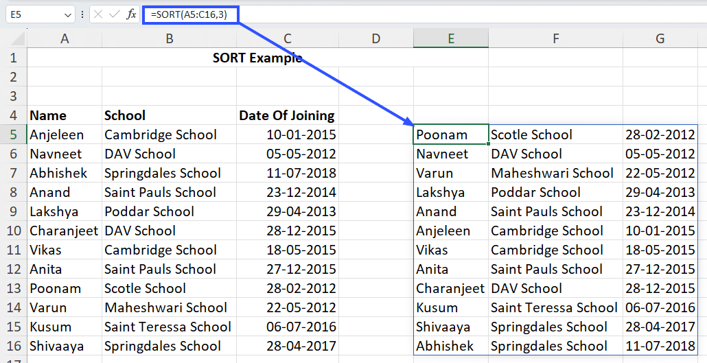
This function returns the whole array, sorted in ascending order of values in the third column (i.e., Date Of Joining).
Sorting By Format: Cell Color, Font Color, Or Icon
If the cells in your data set have different kinds of formatting (cell color, font color, icon, etc.), you can use Excel’s Sort Feature to sort data by formatting.
To do so, follow these steps:
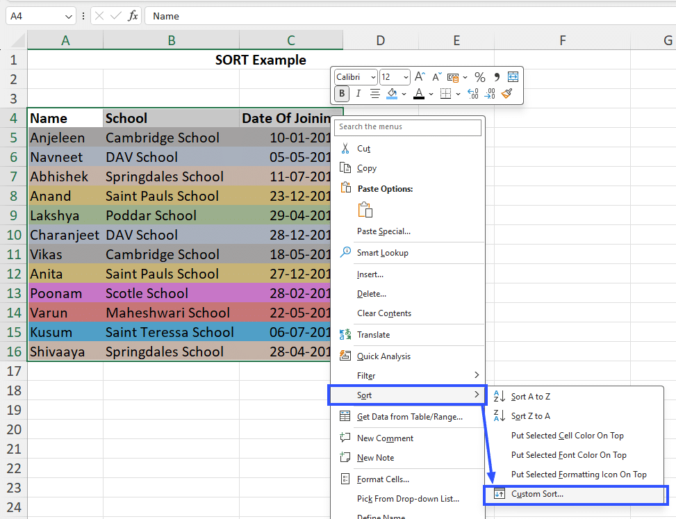
Step 1: Select the range you want to sort (including the column headings).
Step 2: Right-click on the range and select Sort>Custom Sort.
Step 3: In the Sort pop-up window, select Name in the Sort By column Cell Color in the Sort On column.
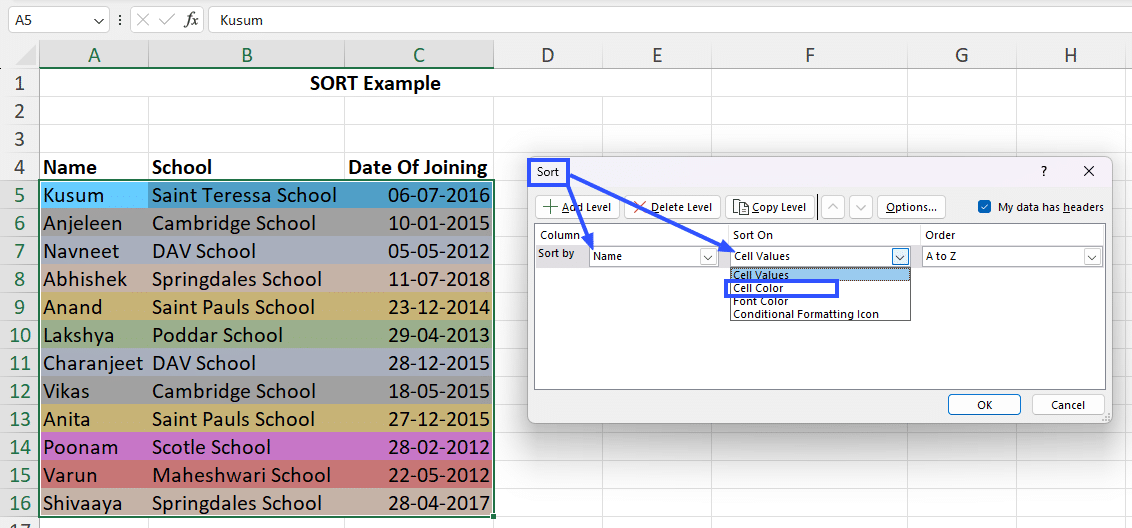
Step 4: In the Order column, select the color you want to appear on top and select the option “On Top”.

Step 5: Click on the “Add Level” button to add the next color in the sorting order.

Step 6: Repeat Step 4 for each color until you reach the desired sorting order.

Step 7: Press the OK button and the range will be sorted based on the color order you chose.
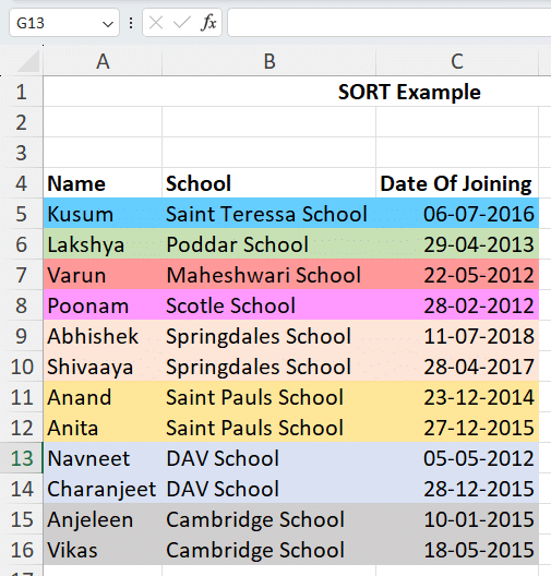
This was an example of sorting by cell color. In the same way, you can sort the array based on Font Color or Conditional Formatting Icon, by choosing it in the Sort On column in the Sort pop-up.
Sorting By Conditional Formatting
If you’ve applied conditional formatting to the range of cells you want to sort, you can use the same steps as in the Sorting By Format Example above.
Let’s say you’ve applied conditional formatting as per:
- Result<30: Red Color
- 30<Result<74: Yellow Color
- Result>74: Green Color

Now, using the steps from the previous example, you can set the Custom Sort order for the range you want to sort.
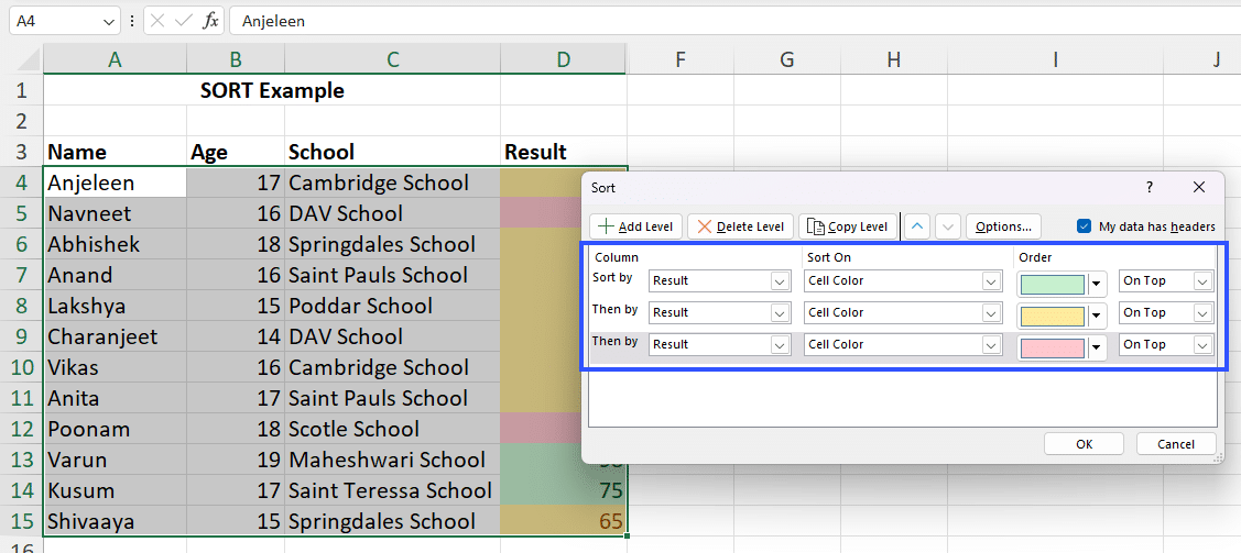
Once you click the “OK” button, your selected range will be sorted according to cell color (Green>Yellow>Red).

Sorting Data Using A Custom List
If you want to sort an array based on certain values in a column, instead of plain ascending/descending order, you’ll have to use a custom list.
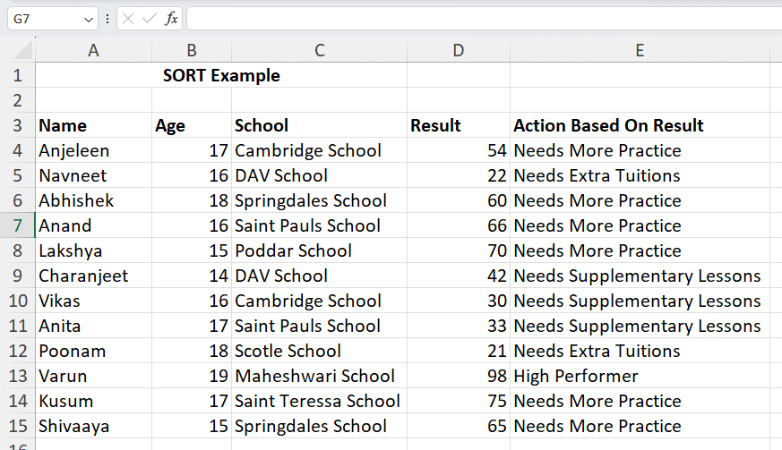
For example, you want to sort a list of students based not on their score, but on the Action based on their Result, regular SORT won’t work.
In this case, you can create a custom list which is presorted in the order you want. Here are the steps to do it.
Creating A Custom List
Step 1: List the unique values from column E in a separate column, sorted in the order you want your original array to be sorted in.
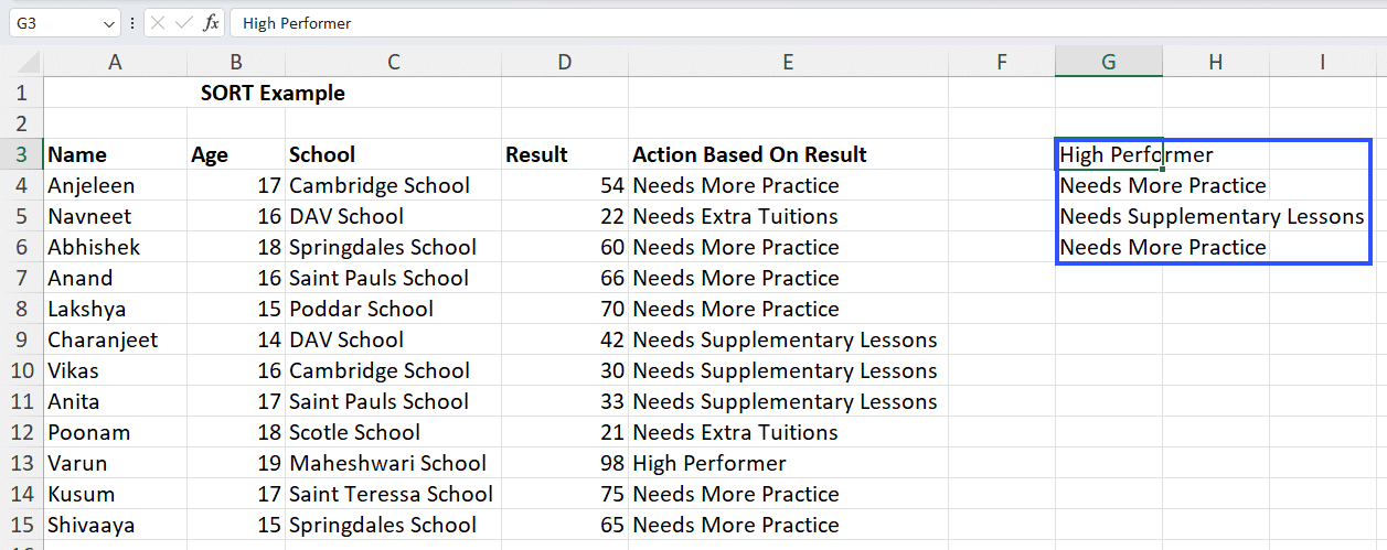
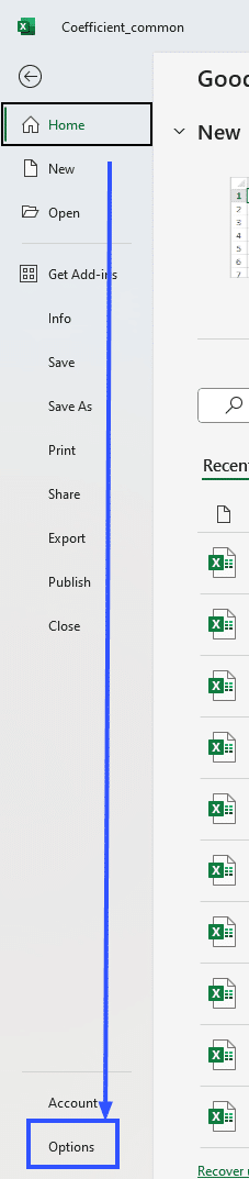
Step 2: Select all the cells G3:G6, which contain the list of unique values from column E. Click on “File” and then “Options”.

Stop exporting data manually. Sync data from your business systems into Google Sheets or Excel with Coefficient and set it on a refresh schedule.
Get Started

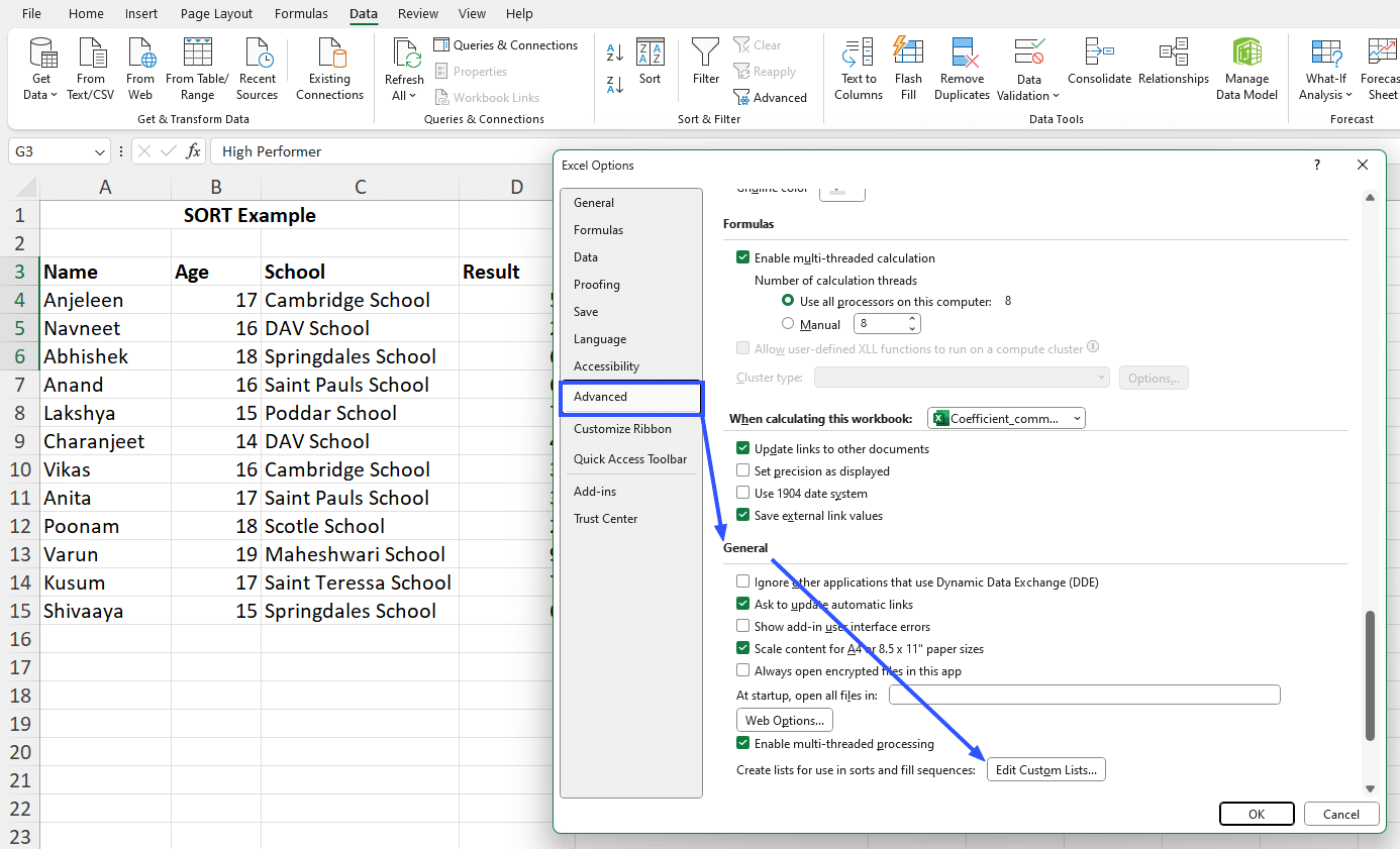
Step 3: In the options pop-up window, select “Advanced”, then scroll down to the “General” section and click on “Edit Custom Lists”.
Step 4: Since you’d already selected the cells containing the presorted values, the range will appear in the “Import list from cells:” field. So just press the “Import” button.

Step 5: A new list will appear in the Custom Lists column with the List Entries fields pre-populated based on the cells you selected in Step 1. Now, click on the “OK” button.

Step 6: Excel will take you back to the “Advanced” tab in the Options pop-up window. Just click the “OK” button.

This concludes the creation of the custom list.
Sorting Data Based On The Custom List
Next, to sort your desired range based on this custom list, follow these steps:
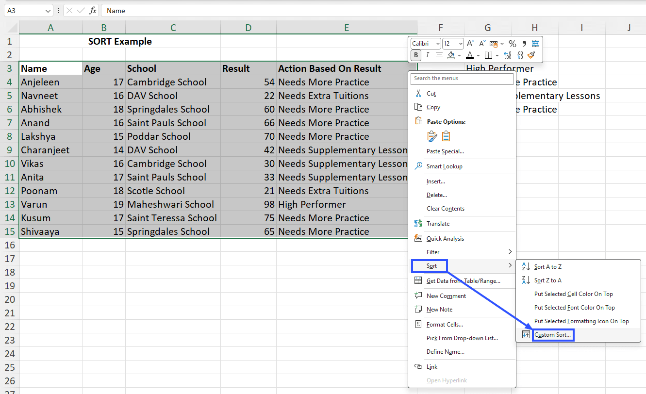
Step 1: Select your desired range of cells and right-click on the selection. Then select “Custom Sort” from the “Sort” drop-down menu.
Step 2: In the Sort pop-up window, select the column you want the range to be sorted by. In this case, the Action Based On Result column.
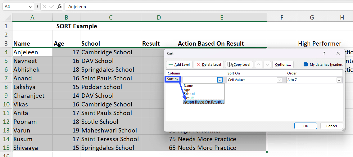
Step 3: The default value of the Sort On column is Cell Values, so leave it as it is. But for the Order column, select the Custom List option from the drop-down menu.

Step 4: This will bring up the Custom Lists pop-up window, where you can select the custom list you created earlier, then click the “OK” button.

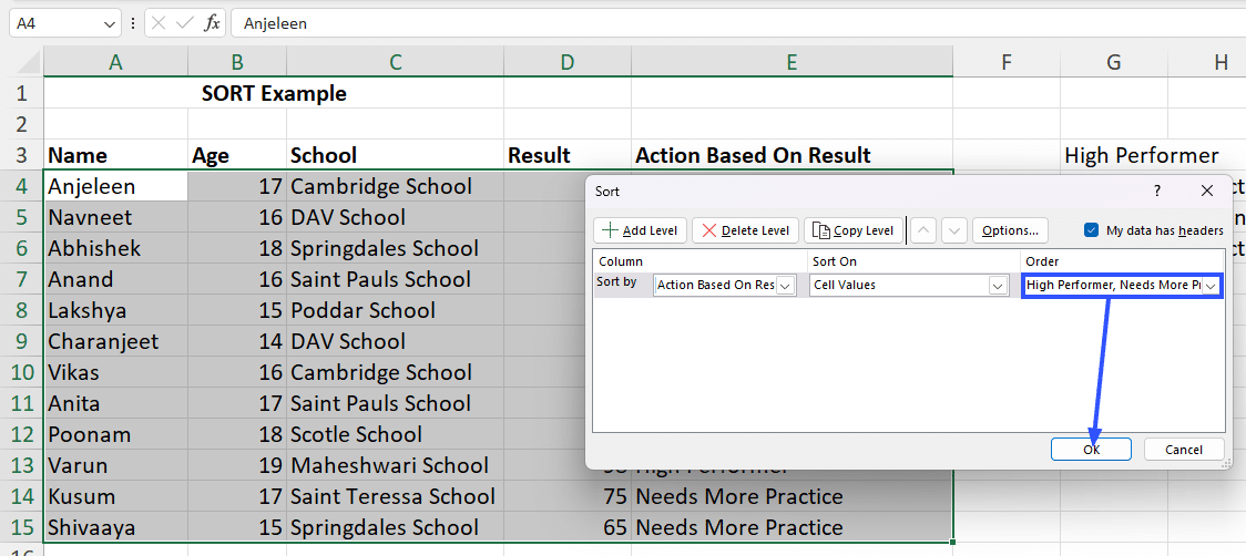
Step 5: Excel will take you back to the Sort pop-up window, where you can see the custom list has appeared in the Order column. Now, click the “OK” button.
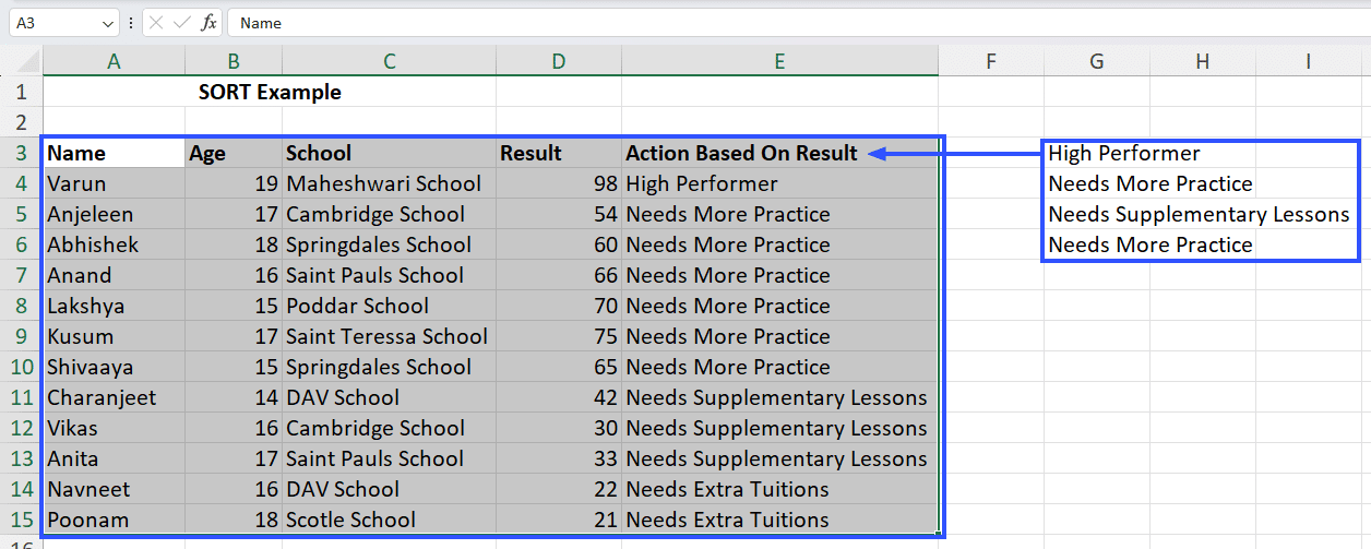
Step 6: Your desired array is now sorted by the values in the Action Based On Result column, based on which we created the custom list.
Sorting Based On Specific Criteria
You can use FILTER to set a criteria (or multiple criteria) and combine it with the Excel SORT function to sort the filtered results.
The formula to use is: =SORT(FILTER(A4:E15,D4:D15>H3),4)

This function filters the range A4:E15 which matches the criteria that the value in the Result column should be >30. Then it sorts the filtered range in ascending order of the values in the fourth column of the original array, i.e., Result.
We’ve covered a lot of use cases of the Excel SORT function, but we haven’t yet talked about what happens when you run into errors while using it. So let’s dive into that.
Troubleshooting Common Issues When Using Excel SORT Function
Let’s talk about troubleshooting some common errors when using the Excel SORT function:
- #SPILL! Error
The #SPILL! error occurs when there’s a non-blank cell in the way of the output array To fix it, make sure all the cells that will be occupied by the output array are blank.
Another thing to note is that merged cells (even if they’re blank) can cause the #SPILL! error, so make sure there are no merged cells in the way of the output. - #NAME? Error
The most common reason for this error is a misspelled function name, so fixing it should get rid of this issue.
Sometimes, you can also run into this error when your version of Excel doesn’t support the SORT function, in which case, update your software or use the web version. - #Value! Error
This error can occur when you use the wrong type of arguments or are trying to execute an operation that conflicts with the valid data types (like multiplying two text strings). Getting rid of these issues should fix the #Value! error. - #REF! Error
The most common reason for this type of error is when the function references cells or worksheets that have been removed. So check your arguments to ensure that you’re using valid references. - #N/A Error
This error occurs when the SORT function can’t locate the data to sort or the specified range indulges non-numeric or non-text entries that can’t be stored. So, ensure that the range you are trying to sort contains data. - #NULL! Error
This error derives when the SORT function extracts an incorrect range or the stated range has a space between references, causing the formula to consider it invalid. So, correct any mistyped cell addresses. - #SPILL! Error with Dynamic Arrays
This error occurs when a SORT function is a part of a dynamic array that tries to disclose into a range engaged by other data or hindered by combined cells. So, avoid using combined cells in the spill range.
Other than these errors, which often have a straightforward reason, there could be some issues where the Excel SORT function doesn’t behave as expected. Let’s tackle those next.
Managing Unexpected Sorting Results
If the SORT function doesn’t behave as expected, here are some tips to help you deal with the issue:
- Set Excel to Automatic Computation: Make sure that your workbook is set to automatic computation. You can find this under Formulas > Calculation Options.
- Unhide Rows and Columns: Make sure that there are no hidden rows or columns in the data, which can result in unexpected outcomes.
- Check your Local Excel Settings: Sorting can be impacted by local settings, specifically for date and currency structures. Make sure that your system’s local settings match the data structure.
- Including/Excluding Headers: Ensure to check the option to include or exclude headers from your data set when using the Excel SORT Function. Misapplying this can result in headers being sorted along with data.
- Check for Merged Cells: Merged cells can cause issues with sorting. Unmerge all merged cells in your data before sorting to ensure accurate results.
- Verify Data Types: Ensure that your data is correctly formatted with the appropriate data types (e.g., text, numbers, dates). Excel may not sort data correctly if it is not formatted properly.
- Check for Leading Spaces: Leading spaces in cells can affect sorting results. Use the TRIM function to remove leading and trailing spaces before sorting.
Even after taking these precautions, If you still encounter unexpected sorting results, use the “Undo” option (Ctrl + Z) and try a different approach.
There is one more thing to keep in mind about the Excel SORT function.
Availability Of SORT In Different Excel Versions
Excel SORT Function is completely supported in Office 365 which has Dynamic Arrays permitted by default. This means that formulas that return multiple values (like SORT) will spontaneously spill over into adjoining cells.
However, the Dynamic Arrays feature is not supported in Excel 2019. Features like Excel SORT, FILTER, and others that output arrays are not available.
Also note, Excel 2019 is a static version, which means it cannot get new functions after its original release, unlike the constantly updated Office 365. So if you want to utilize SORT, make sure you’re using the latest version of Excel.
Now that we’ve got that sorted, let’s wrap this up.
Using The Excel SORT Function
The Excel SORT function can come in handy for quickly and easily organizing your data. Whether you need to sort a list of names, numbers, dates, or even across multiple columns, the SORT function makes it simple.
When combined with other functions and features, the Excel SORT function can help you organize and structure your data exactly the way you want.
We’ve also discussed the shortcomings of SORT when dealing with improperly formatted data and missing references. These situations will often come up when dealing with multiple dynamic worksheets.
So to make your life easier, say hello to Coefficient, the leading spreadsheet automation tool which can help you connect all your data sources, automate workflows, and share live insights within Excel. Get started today.


