Introduction To The Excel Match Function
The Excel MATCH function can help you quickly locate the position of a specific value within a range of cells. But it is rarely used by itself because combining it with other functions can help you sort, filter, and find the exact data points you want.
Want to learn in what ways you can use the Excel MATCH function? You’re in the right place.
In this article, we will walk you through the integrals of the MATCH function, complete with practical instances and formulas. By the end of this guide, you will be able to effectively find the data in your spreadsheets and incorporate MATCH with other Excel functions for maximum workflow.
But first, let’s examine the syntax and arguments needed for the MATCH function to do its job.
Excel MATCH Formula Syntax
The syntax for using the MATCH function is: =MATCH(lookup_value, lookup_array, [match_type])
Let’s look at each parameter in a little more detail:
- lookup_value is the value you’re trying to find in an array.
- lookup_array is the range of cells you’re searching within.
- match_type is an optional argument that determines how the function will find the match. This value can be:
- 1 for finding the closest match below in the lookup_array that is less than or equal to the lookup_value. This is the default value and requires the array to be sorted in ascending order.
- 0 for an exact match. This will find the first exact match in the array.
- -1 for finding the closest match above that is greater than or equal to the lookup_value. This requires the array to be sorted in ascending order.
The function will return a number, which indicates the relative position of the lookup_value in the range defined by lookup_array. However, if no match is found, the function will return the #N/A error.
With the syntax clarified, let’s see some simple examples of the Excel MATCH function in action.
Examples Of Using The Excel MATCH Function
Example #1: Closest Match Below
Let’s assume we have a list of 10 names, which we’ve sorted alphabetically in ascending order. To find the closest match below to the name “Ethan” in this array, use the formula: =MATCH(J3,G4:G13,1)
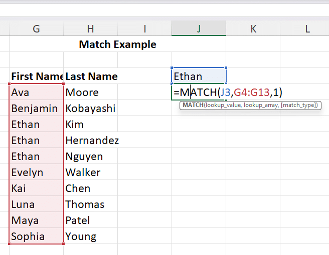
This will return the value 5, as this is the position of the “closest match below” in the array
- We’ve used J4 as the lookup_value, but we could use “Ethan” as well.
- The lookup_array is G4:G13 as this contains all the first names.
- The match_type is 1. Or we could have just left it undefined as it’s the default value.
Note: If the array wasn’t sorted or sorted in ascending order, you’d get the #N/A error. So please double check that when using this match type.
Example #2: Exact Match
To find the exact match to the name “Ethan” in this array, use the formula: =MATCH(D3,A4:A13,0)
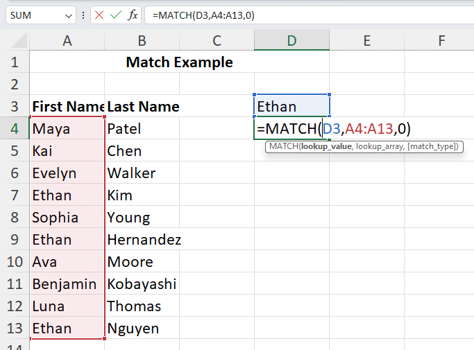
This will return the value 4, as this is the position of the first occurrence of the exact match in the array.
Note: The array isn’t sorted, but there’s no error as the exact match type doesn’t require a sorted array.
Example #3: Closest Match Above
To find the closest match below to the name “Ethan” in this array, use the formula: =MATCH(P3,M4:M13,-1)
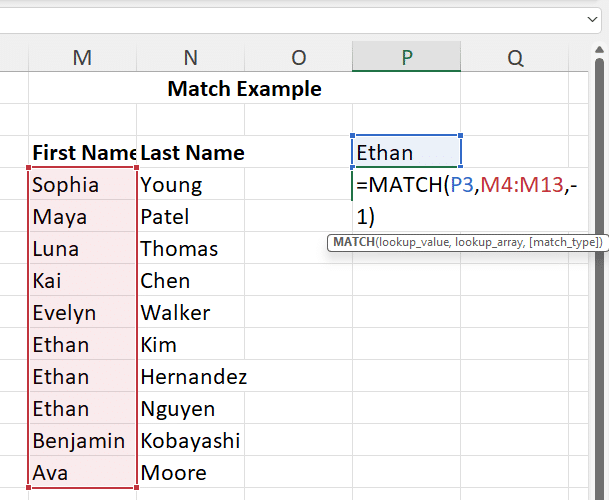
This will return the value 6, as this is the position of the “closest match above” in the array, which is sorted in descending order.
With these examples out of the way, let’s dive into some more practical use cases of the Excel MATCH function.
Video Tutorial
Check out the tutorial below for a complete video walkthrough!
More Practical Examples Of Using The Excel MATCH Function
Let’s look at some more examples of how to use the MATCH function for some practical use cases.
Practical Example #1: Partial Match With Wildcards
You can use the wildcards ? (question mark) and * (asterisk) for partial text matches in a list.
Let’s say you’re a teacher and have a list of names of students in your sheet. You want to make a comment against a student’s name, recommending them for a high performer award, but you can’t remember their exact name.
However, you do recollect that their last name starts with a ‘Ko.’ In this case, you can use the asterisk wildcard (*) to search for last names starting with ‘Ko*’ to find the student you’re looking for.
The formula you’d use to find this name is: =MATCH(D3,B4:B13,0)
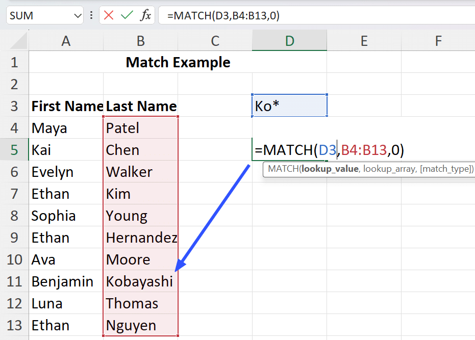
This will return the value 8, corresponding to the last name ‘Kobayashi,’ which is the eighth name in the list.
Similarly, you can use the question mark wildcard (?) to search for a name whose spelling you’re unsure of.
Practical Example #2: Case-Sensitive Matches
By default, the Excel MATCH function is case-insensitive. So if you want to find a case sensitive match, you have to combine MATCH with the EXACT function.
Let’s say you’re doing an inventory, and some product codes are only differentiated by an upper/lower case letter.
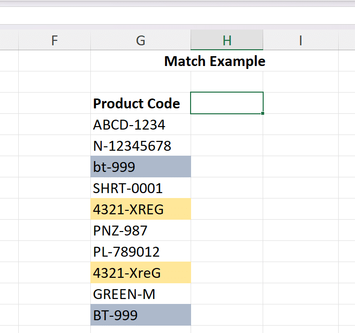
If you were to use the standard MATCH function syntax, you’d only get the first instance of the product codes highlighted above. I.e., 3 and 5.
But you can get an exact match by combining the MATCH function with the EXACT function like this: =MATCH(TRUE,EXACT(G4:G13,I3),0)
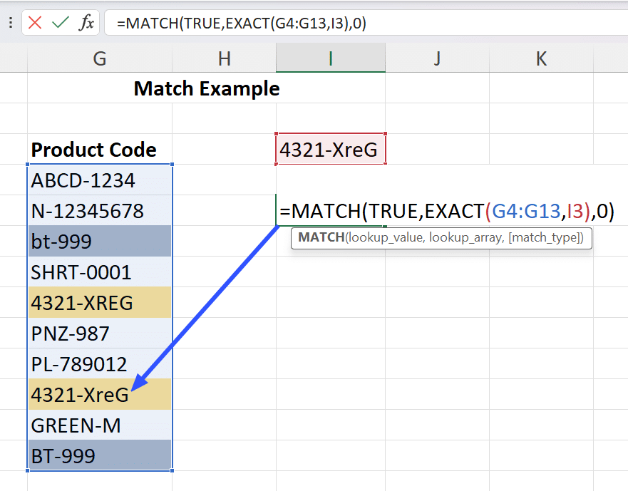
Cell I3 contains the exact (case-sensitive) product code. So the EXACT function compares it to all the entries in the range G4:G13 and returns the value ‘TRUE’ only in case of an exact match. The MATCH function then returns the relative position of this exact match in the list, which, in this case, is 8.
Practical Example #3: Comparing 2 Columns For Matches And Differences Using ISNA MATCH
If you have to compare two lists and find which entries are present in both lists, you can use the ISNA MATCH function.
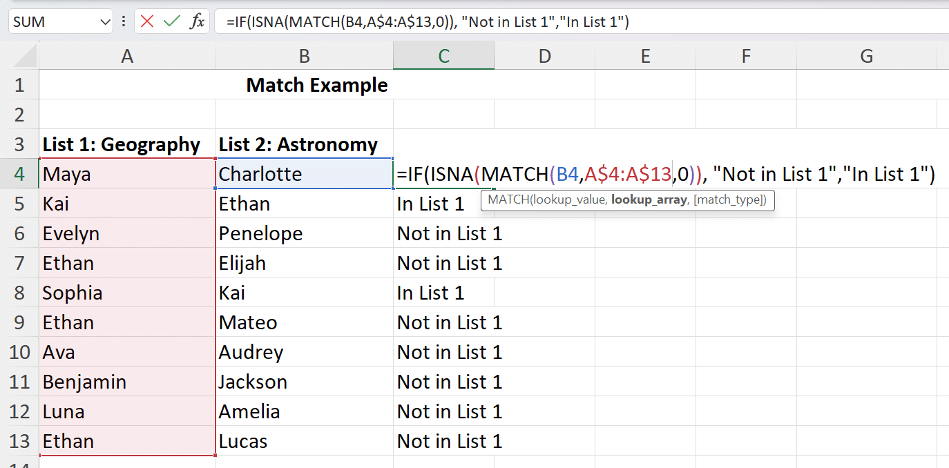
Let’s say List 1 contains names of students who performed well in Geography and List 2 has names of those who performed well in Astronomy.
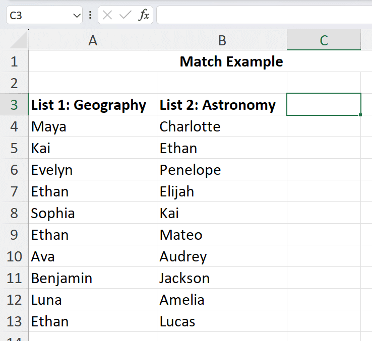
To find out which names are present in both lists, you’d use the ISNA function (which returns TRUE/FALSE based on whether there is an #N/A error) and combine this with the MATCH function (which returns an #N/A error when there is no match).
The syntax would look like: =ISNA(MATCH(B4,A$4:A$13,0))
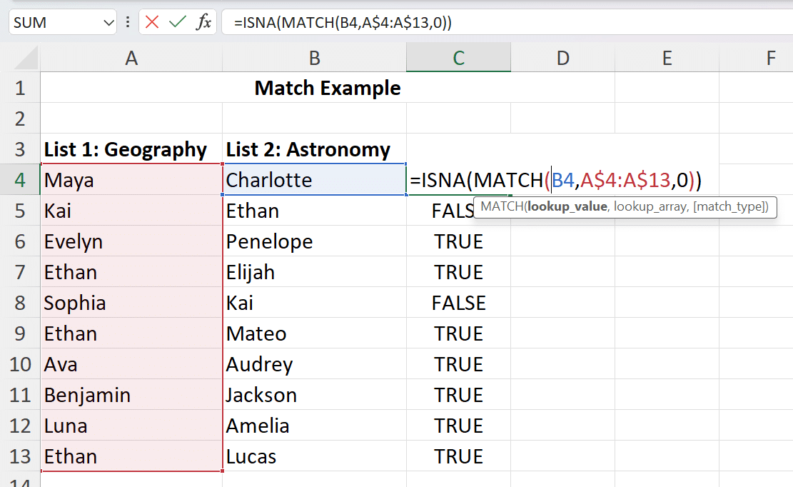
This function returns the value ‘TRUE’ when the name in List 2 is not present in List 1, and ‘FALSE’ when the name in List 2 is also present in List 1. This might seem a little counterintuitive.
So, we’ll use the IF function to make the output simpler to read. The function will now be: =IF(ISNA(MATCH(B4,A$4:A$13,0)), “Not in List 1″,”In List 1”)
This will convert all ‘TRUE’ values to ‘Not in List 1’ and all ‘FALSE’ values to ‘In List 1.’

Stop exporting data manually. Sync data from your business systems into Google Sheets or Excel with Coefficient and set it on a refresh schedule.
Get Started
Practical Example #4: Making VLOOKUP And HLOOKUP More Dynamic With The Excel MATCH Function
If you’ve used the VLOOKUP/HLOOKUP function before, you know that it only works well on a table until you add or delete a row/column. This is because the col_index_num/row_index_num argument changes when you add or delete a column/row in the defined table. But the table_array argument remains unchanged.
For e.g., in the table below, we want to see Ethan’s Geography score. So we use the VLOOKUP function: =VLOOKUP(F3,$A$3:$C$13,2,FALSE)
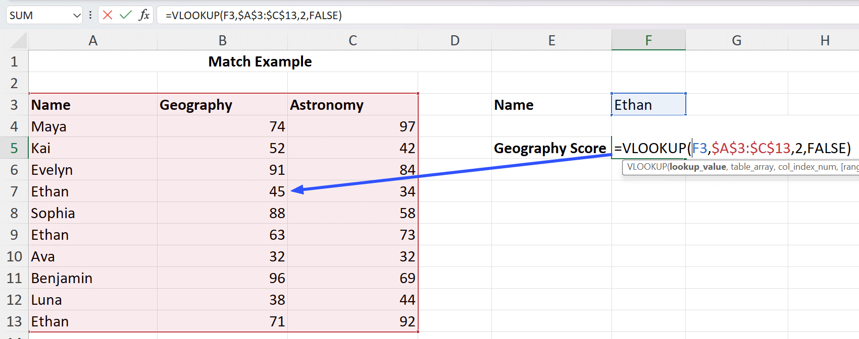
This will return the value 45.
However, if you inserted or deleted a column in the table, it would change the col_index_num argument, resulting in an incorrect output or an error.
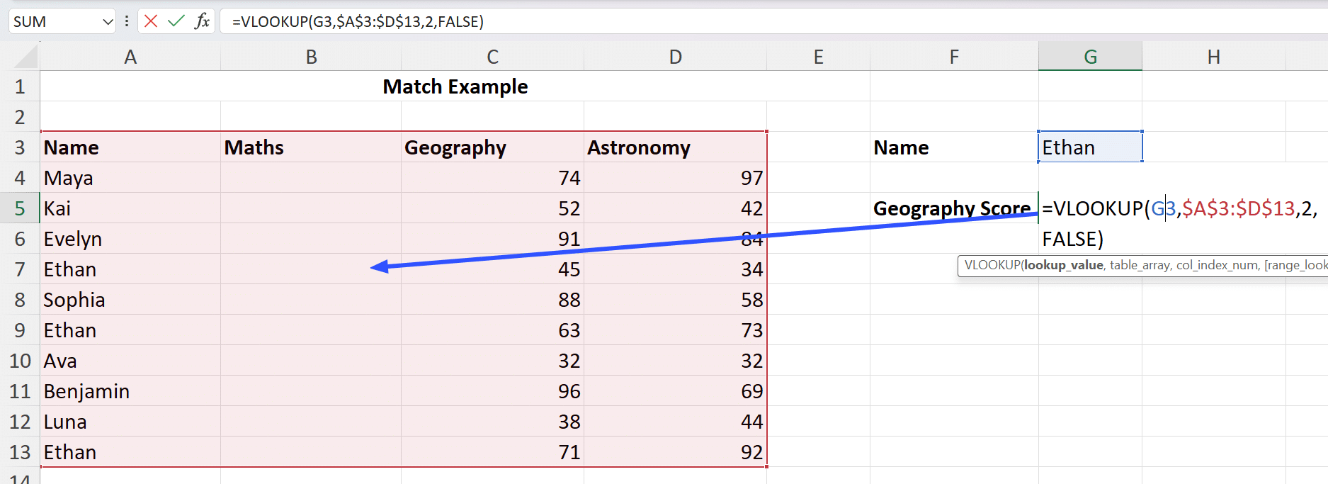
This function will return to value 0.
To overcome this shortcoming, you can use the Excel MATCH function to define the col_index_num argument like so: =VLOOKUP(G3,$A$4:$D$13,MATCH($F$5,$A$3:$D$3,0),FALSE)
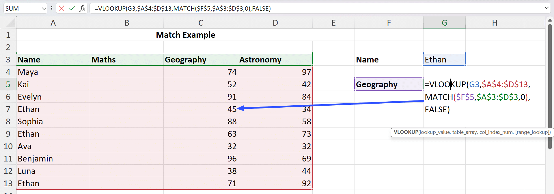
This function will return to value 45.
All we did was, instead of giving an absolute value for the col_index_num argument, we used the MATCH function to look up the subject name in cell F4 in the array containing all the subject names (A3:D3) and return the matching column number.
Similarly, you can modify the HLOOKUP with the Excel MATCH function to define the row_index_num argument, instead of specifying a particular row number.
That covers most of the common use cases of the function MATCH in Excel. So let’s sum it up.
Common Errors and Troubleshooting Tips for the MATCH Function
Using the Excel MATCH Function can substantially improve your data search abilities. However, like any function, it can sometimes generate errors or unanticipated outcomes. Comprehending these common issues and knowing how to troubleshoot them can save you time and annoyance.
Common Errors
#N/A Error
Cause: When you apply the MATCH Function in a wrong way, it return an error #N/A when it cannot locate the lookup_value in the lookup_array.
Solution: Ensure the lookup_value exists within the lookup_array. If you are utilizing an exact match (match_type = 0), validate the exact value exists, indulging in special characters or spaces.
#VALUE! Error
Cause: The match function generates a #VALUE! Error when the lookup_array isn’t a valid range or if there is a problem with the match_type.
Solution: Examine if the lookup_array is correctly depicted as a range of cells. Also, ensure that the match_type is a valid number (0,1, or -1).
#REF! Error
Cause: This error occurs when the lookup_array contains quotations that are not valid or if the MATCH function is used erroneously in coexistence with other functions such as INDEX.
Solution: Validate that the values you input in the formula are correct and within the pertinent ranges.
Troubleshooting Tips
Check for the Exact Matches with Accuracy
Tip: When using exact matches (match_type = 0), cross-check for hidden characters, extra spaces, or distinct types of data. Utilizing functions such as TRIM() or CLEAN() can help organize your data.
Verify Data Types
Tip: Ensure that the types of data for the lookup_value and lookup_array are compatible. Incompatible data types (e.g., text vs. numbers) can cause error or erroneous outcomes. Use the VALUE () function to alter text to numbers if required.
Use Helper Columns for Intricate Data
Tip: When handling intricate data or multiple norms, consider using the helper columns to simplify the data into a format more appropriate for the MATCH function. This can make your formulas easier to handle and amend.
Check for Duplicates
Tip: Be cognizant that the MATCH function returns the first event of the lookup_value. If duplicates are there in your data, consider using extra functions such as COUNTIF to manage duplicates suitably.
Using The Excel MATCH Function
We hope that this article has helped you understand why and how to use the MATCH function in Excel. With ample examples of the different use cases, you should be able to use the MATCH function to analyze your data as granularly as you desire.
Finding matches in Excel and figuring out how to work it into other functions can be time consuming. Say goodbye to repetitive tasks and hello to efficiency with Coefficient, the leading spreadsheet automation tool trusted by over 350,000 professionals worldwide. Get started today with Coefficient today and alter the way you work with Excel!


