The ISERROR function is a fundamental error-handling tool in Excel that helps identify and manage various types of errors in your spreadsheet calculations. Whether you’re dealing with complex formulas or large datasets, understanding ISERROR is essential for creating robust and reliable spreadsheets. Let’s explore how to implement this function effectively across Excel versions 2021-2024.

How to Use the ISERROR Function in Excel

The ISERROR function checks if a value or expression results in any type of Excel error. Its syntax is straightforward:

=ISERROR(value)

Where ‘value’ can be a cell reference, formula, or direct value you want to check for errors.

Let’s break down the implementation:

1. Open Excel and select the cell where you want to check for errors
2. Type the equals sign (=) to start the formula
3. Enter ISERROR followed by an opening parenthesis
4. Input the value or cell reference you want to check
5. Close the parenthesis and press Enter

Example results:

Formula	Result	Explanation
=ISERROR(A1/0)	TRUE	Division by zero error
=ISERROR(“Text”)	FALSE	No error in text value
=ISERROR(1+1)	FALSE	Valid calculation

Creating Your First ISERROR Formula

Let’s start with a common scenario: handling division by zero errors.

Step 1: Set up your data

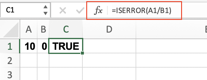
1. Enter a number in cell A1 (e.g., 10)
2. Enter a potential divisor in cell B1 (e.g., 0)

Step 2: Create the formula

1. In cell C1, enter: =ISERROR(A1/B1)
2. Press Enter to see the result

The formula will return TRUE if B1 contains zero (creating a #DIV/0! error) and FALSE if B1 contains any other number.

Combining ISERROR with IF Statements

To make ISERROR more practical, combine it with IF statements to display custom messages:

Formula structure:

=IF(ISERROR(formula), value_if_error, formula)

Example implementation:

Step 1: Create a division formula with error handling

1. In cell C1, enter: =IF(ISERROR(A1/B1), “Cannot divide by zero”, A1/B1)
2. This returns either the calculation result or your custom message

A1	B1	Formula Result
10	0	Cannot divide by zero
10	2	5
10	5	2

ISERROR with VLOOKUP and Common Excel Functions

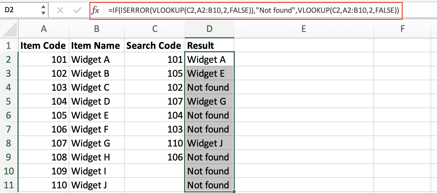
ISERROR is particularly useful when working with VLOOKUP functions:

Step 1: Create a lookup table

1. Set up your data range (A1:B10)
2. Create a lookup value in C1

Step 2: Implement ISERROR with VLOOKUP

1. Enter the formula:

=IF(ISERROR(VLOOKUP(C2,A2:B10,2,FALSE)),”Not found”,VLOOKUP(C2,A2:B10,2,FALSE))

Building Complex ISERROR Formulas

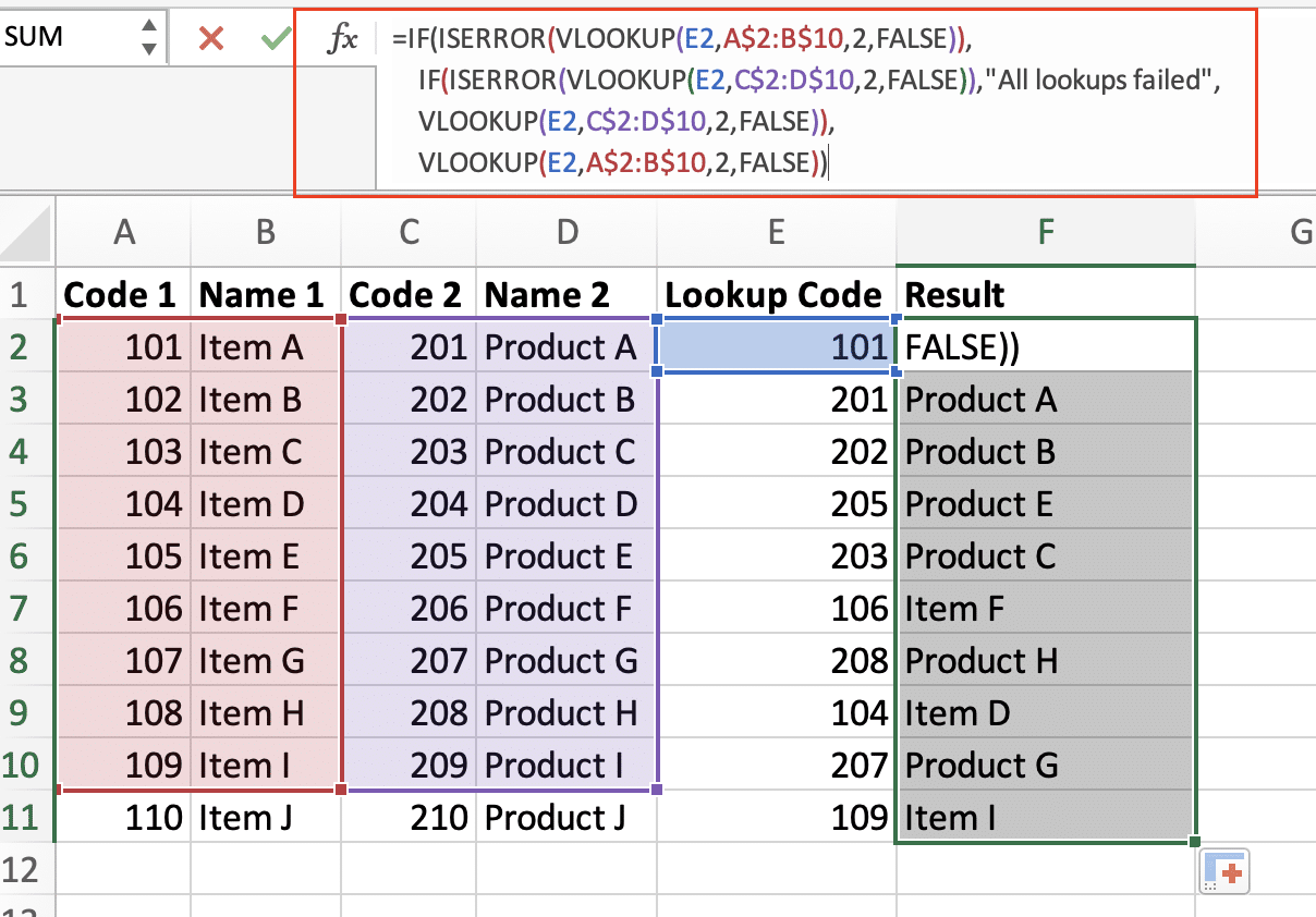
For handling multiple conditions:

Step 1: Create a nested formula

=IF(ISERROR(formula1),

IF(ISERROR(formula2),

“All lookups failed”,

formula2),

formula1)

ISERROR vs IFERROR: When to Use Each

Key differences:

Feature	ISERROR	IFERROR
Syntax Complexity	More complex with IF	Simpler, one function
Performance	Slightly slower	Faster
Flexibility	More control	Less control

ISERROR vs ISERR: Key Differences

ISERROR catches all errors, while ISERR excludes #N/A errors:

Error Type	ISERROR	ISERR
#DIV/0!	TRUE	TRUE
#N/A	TRUE	FALSE
#NAME?	TRUE	TRUE

Error Types and ISERROR Response

Common Excel errors ISERROR detects:

• #DIV/0! (Division by zero)
• #N/A (Value not available)
• #NAME? (Invalid formula name)
• #NULL! (Invalid cell reference)
• #NUM! (Invalid numeric value)
• #REF! (Invalid cell reference)
• #VALUE! (Wrong value type)

Putting It All Together

ISERROR is essential for creating robust Excel formulas that handle errors gracefully. Start with simple implementations and gradually build more complex solutions as needed. Remember to test your formulas with various scenarios to ensure they handle all potential errors appropriately.

Ready to take your Excel data handling to the next level? Try Coefficient to seamlessly sync live data from 50+ business systems directly into your spreadsheets. Get started with Coefficient today and eliminate manual data entry errors while keeping your spreadsheets automatically updated with real-time data.