Excel Header Tutorial: Add, Edit & Manage Headers Like a Pro (2024)

Want to create professional-looking Excel spreadsheets with well-organized headers? This guide walks you through adding, customizing, and managing headers in Excel.

How to Add a Header in Excel

Headers in Excel help organize your data and make your spreadsheets more readable. Here’s how to add them:

Step 1: Open your Excel spreadsheet.

• Launch Microsoft Excel and open the workbook where you want to add a header.
• If you’re starting from scratch, create a new workbook.

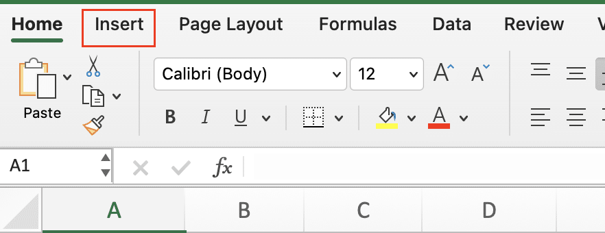
Step 2: Navigate to the “Insert” tab on the ribbon.

• Look for the ribbon at the top of your Excel window.
• Click on the “Insert” tab to reveal its options.

Step 3: Click on “Header & Footer” in the Text group.

• Find the “Text” group within the “Insert” tab.
• Click on the “Header & Footer” button.

Step 4: Excel switches to Page Layout view automatically.

• Your spreadsheet view will change to show the header area.
• You’ll see placeholder text boxes for left, center, and right sections of the header.

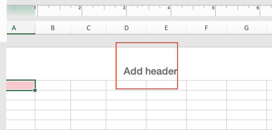
Step 5: Type your desired header text in the top section.

• Click on any of the three header sections (left, center, or right).
• Type the text you want to appear in your header.

Customizing Header Content

Once you’ve added a basic header, you can enhance it with various elements:

Using Built-in Codes for Dynamic Information

Excel provides codes to insert automatically updating information:

Step 1: Place your cursor where you want the dynamic content.

• Click in the header section where you want to add the information.

Step 2: Click on the “Header & Footer Elements” in the Design tab.

• This tab appears when you’re editing headers and footers.

Step 3: Choose the type of information you want to insert.

• Options include:
  • Page Number: &[Page]
  • Number of Pages: &[Pages]
  • Current Date: &[Date]
  • Current Time: &[Time]
  • File Path: &[Path]&[File]
  • File Name: &[File]
  • Sheet Name: &[Tab]

Step 4: The code will appear in your header.

• Excel will display the actual information when you exit header editing mode.

Inserting Images or Logos into Your Header

Adding visual elements can make your headers more professional:

Step 1: Click where you want to insert the image in your header.

• Position your cursor in the left, center, or right header section.

Step 2: Click on the “Picture” button in the Header & Footer Elements group.

• This opens a file browser window.

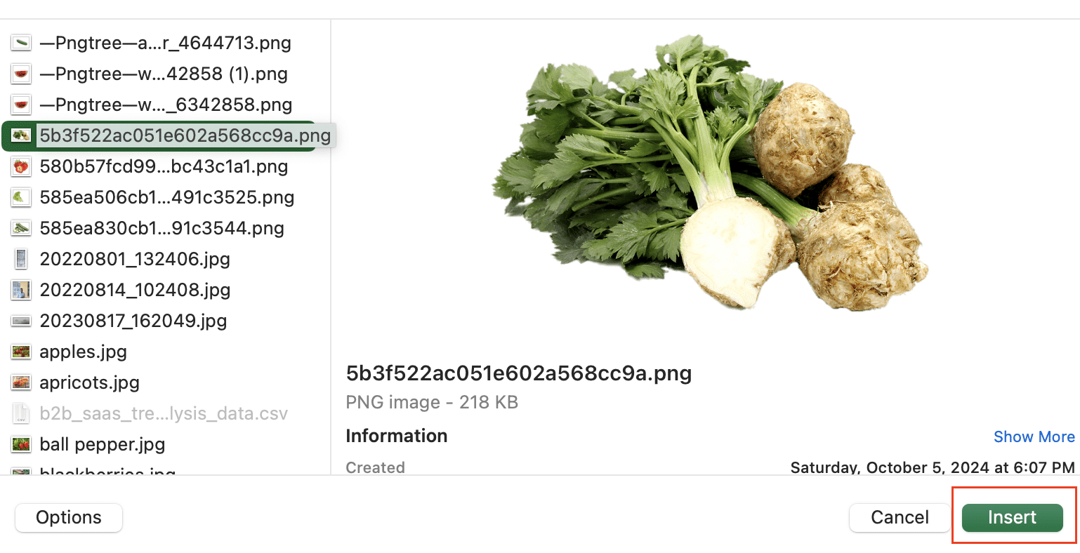
Step 3: Select the image file you want to use.

• Navigate to the location of your logo or image file.
• Click “Insert” to add it to your header.

Step 4: Adjust the image size if needed.

• Use the sizing handles to resize the image within your header.

Applying Text Formatting Options to Header Content

Customize the look of your header text:

Step 1: Select the text you want to format in your header.

• Highlight the text by clicking and dragging your cursor over it.

Step 2: Use the Mini Toolbar or Format Cells dialog.

• Right-click the selected text to access formatting options.
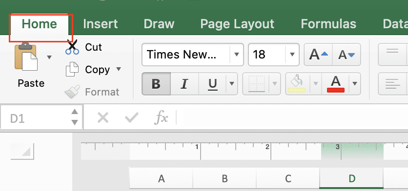
• Or use the “Home” tab on the ribbon for more formatting choices.

Step 3: Apply desired formatting.

• Change the font, size, color, or style (bold, italic, underline).

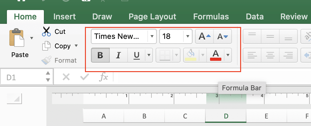
• Adjust alignment or add effects as needed.

Creating Different Headers for Odd and Even Pages

For documents with facing pages, you might want different headers:

Step 1: Access the “Header & Footer Tools” contextual tab.

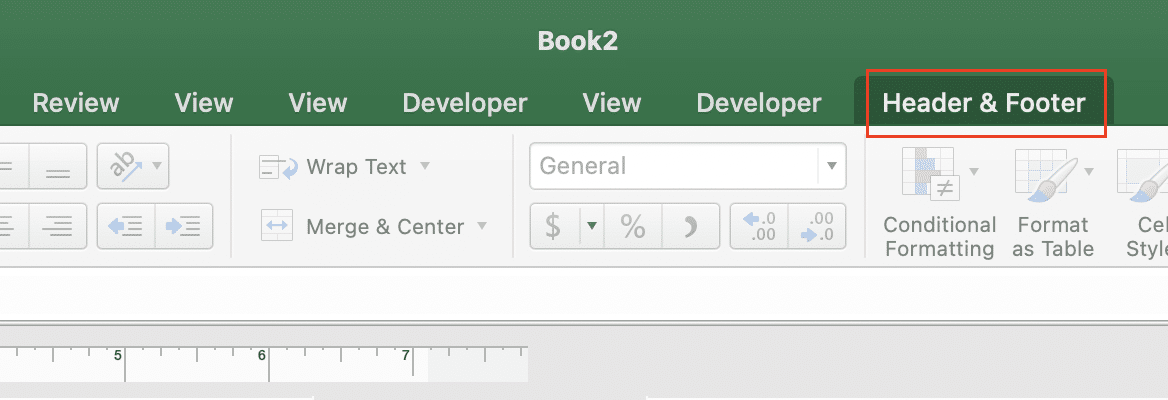
• This tab appears when you’re in header editing mode.

Step 2: Check the “Different Odd & Even Pages” option.

• Look for this checkbox in the “Options” group of the Design tab.

Step 3: Edit headers separately for odd and even pages.

• You’ll now see “Odd Page Header” and “Even Page Header” sections.

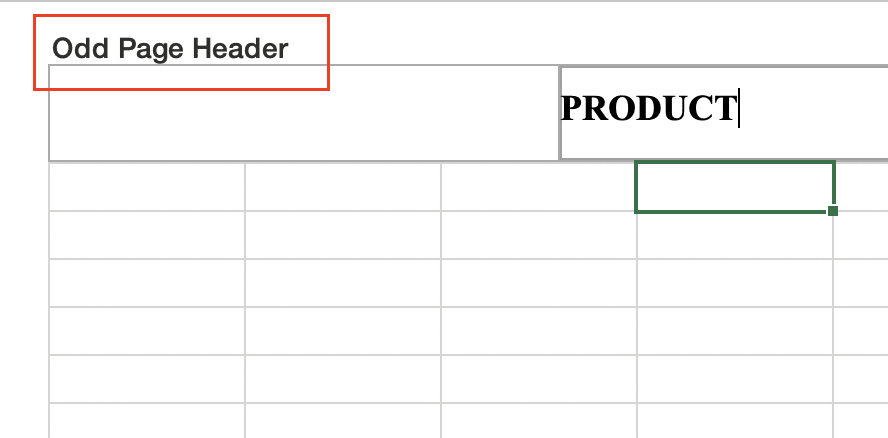
• Customize each as needed, following the steps from earlier sections.

Managing Header Rows in Excel Tables

Excel tables offer special header functionality:

Step 1: Select your data range.

• Highlight the cells you want to include in your table.

Step 2: Click “Insert” > “Table” on the ribbon.

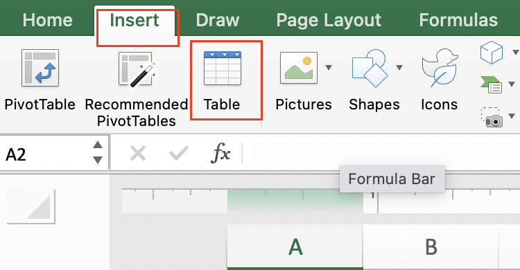
• This opens the “Create Table” dialog box.

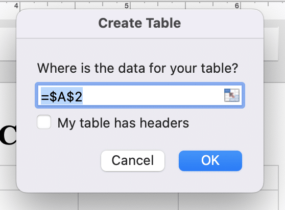
Step 3: Ensure “My table has headers” is checked.

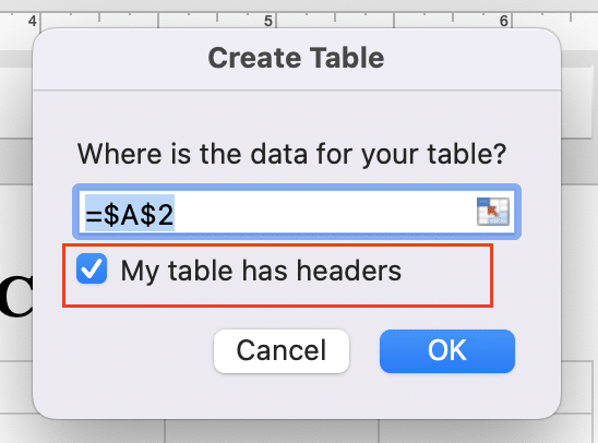
• This option is usually at the bottom of the dialog box.
• If your first row contains column names, make sure this is selected.

Step 4: Click “OK” to create the table.

• Your data is now formatted as an Excel table with headers.

Step 5: Use the “Table Design” tab to toggle header row visibility.

• This tab appears when you select any cell within your table.

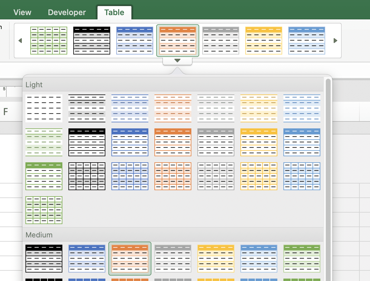
• Look for the “Header Row” checkbox in the “Table Style Options” group.

Freezing Header Rows for Easy Navigation

Keep your headers visible while scrolling through large datasets:

Step 1: Select the row below your header.

• Click on the row number just below your header row.

Step 2: Go to “View” > “Freeze Panes” > “Freeze Top Row”.

• Find this option in the “Window” group of the “View” tab.

Step 3: Scroll through your data while keeping the header visible.

• Your header row will now stay in place as you move through the spreadsheet.

How to Format Headers in Excel Cells

Create visually distinct headers within your spreadsheet:

Step 1: Select the cells you want to use as headers.

• Highlight the row or cells that will serve as your header.

Step 2: Apply desired formatting.

• Use the “Home” tab to access formatting options:
  • Click the “Bold” button (Ctrl + B) for emphasis.
  • Use “Center Align” to center your header text.
  • Click “Fill Color” to add a background to your header cells.

Step 3: Use conditional formatting for dynamic header styles.

• Go to “Home” > “Conditional Formatting” for more advanced options.

• Create rules that change header appearance based on cell content or other criteria.

Creating Header Templates for Consistency

Save time by creating reusable header formats:

Step 1: Design your preferred header format.

• Set up your spreadsheet with the desired header style and layout.

Step 2: Save the workbook as a template.

• Click “File” > “Save As“.

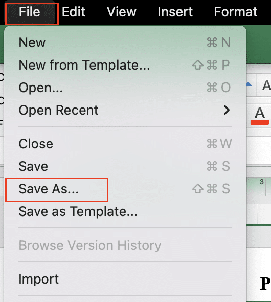
• Choose “Excel Template (*.xltx)” from the file type dropdown.

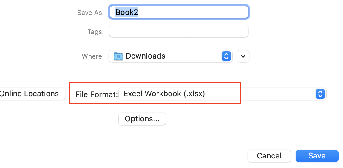
• Name your template and save it in the default template location.

Step 3: Use the template for new spreadsheets.

• When creating a new workbook, select “New from Template“.

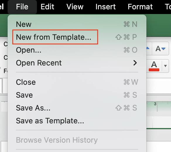
• Choose your saved header template to start with pre-formatted headers.

Adjusting Header Display Options

Control how and when your headers appear:

Step 1: Switch between Normal, Page Layout, and Page Break Preview.

• Use the view buttons at the bottom right of your Excel window

.

• Or go to the “View” tab and select your preferred view.

Step 2: Customize header visibility in different Excel views.

• Headers are typically visible in Page Layout view.
• They may not show in Normal view unless you’re actively editing them.

Step 3: Modify print settings to control header appearance on printed pages.

• Go to “File” > “Print” to access print settings.

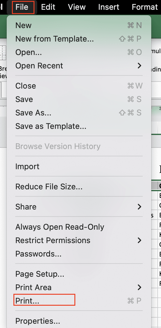
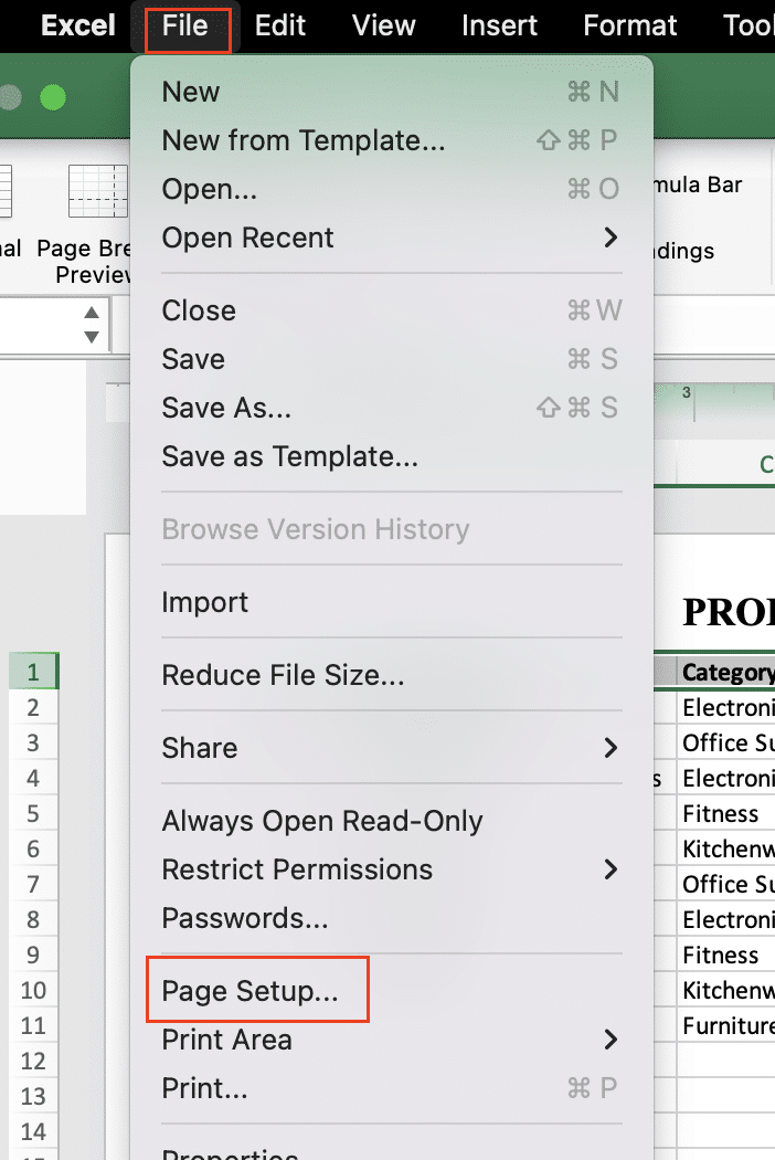
• Use “Page Setup” to adjust header placement and scaling for printing.

Enhancing Your Excel Skills

By mastering Excel headers, you’ve improved your spreadsheet organization and presentation skills. Keep exploring Excel’s features to become even more proficient in data management.

Ready to take your Excel skills to the next level? Coefficient can help you seamlessly integrate live data from various sources directly into your spreadsheets. Get started with Coefficient today and transform how you work with data in Excel.