
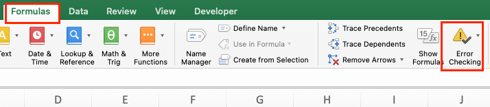
Click the “Formulas” tab in Excel ribbon, then click the “Error Checking” button in the Formula Auditing group
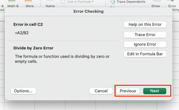
Review errors in the Error Checking dialog box and use “Next” and “Previous” buttons to navigate between error cells
Read error messages carefully to identify the issue (like misspelled function names or divide-by-zero errors)
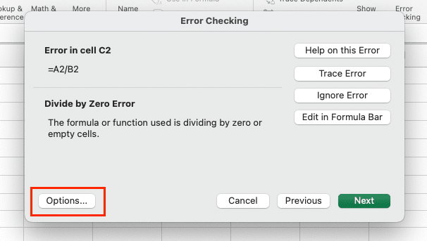
Customize error checking by clicking “Options” button, enabling background error checking, and selecting which error types to include/exclude
Adjust visual indicators by changing the error indicator color from the default green triangles in Excel Options
Excel’s built-in error checking tools make it easy to identify and resolve formula issues quickly, saving you time and frustration. In this comprehensive tutorial, we’ll walk you through how to use Excel’s error detection features to find and fix common spreadsheet errors like #DIV/0!, #NAME?, and #REF!. By the end, you’ll be an expert at using error checking to keep your spreadsheets accurate and error-free.
How to Use Excel’s Error Checking Tool
Excel’s Error Checking tool is a powerful way to find and resolve formula errors across your entire spreadsheet. Here’s how to access and use it:
Accessing the Error Checking Dialog
- Click on the “Formulas” tab in the Excel ribbon.
- In the “Formula Auditing” group, click the “Error Checking” button (it looks like a green checkmark with an exclamation point).

- The Error Checking dialog box will open, displaying the first cell with an error.
Navigating Through Multiple Errors
- Use the “Next” and “Previous” buttons in the Error Checking dialog to move between cells with errors.

- To quickly jump to the next error, you can also press Alt+Shift+F8 on your keyboard.
- Press Alt+Shift+F7 to move to the previous error.
These keyboard shortcuts make it fast and easy to navigate through multiple errors without having to use your mouse.
Using Keyboard Shortcuts for Faster Error Checking
In addition to the navigation shortcuts mentioned above, there are a few other key combinations that can speed up your error checking process:
|
Shortcut |
Action |
|---|---|
|
Alt+Shift+F8 |
Move to next error |
|
Alt+Shift+F7 |
Move to previous error |
|
Alt+F8 |
Open the Error Checking dialog |
|
Alt+Shift+F9 |
Calculate worksheets |
Memorizing these shortcuts will allow you to fly through your error checking routine and make light work of even the gnarliest spreadsheets.
Check Individual Cells for Errors
Sometimes you may want to check a specific cell or range for errors, rather than reviewing the entire spreadsheet. Here’s how:
Selecting Specific Cells with Errors
- Click on the cell you want to check, or drag to select a range of cells.
- Press Alt+F8 to open the Error Checking dialog directly to that cell.
Excel will display any errors found in the selected cell(s).
Using the Error Checking Button
- Select the cell(s) you want to check.
- Click the “Error Checking” button in the Formula Auditing group on the Formulas tab.
- If the selected cell contains an error, the Error Checking dialog will open with details.
This is useful for spot-checking formulas as you build out your spreadsheet.
Reading and Interpreting Error Messages
When the Error Checking dialog identifies a cell with an error, it provides some key pieces of information:
- The cell address of the error
- A description of the error type (e.g. “#DIV/0!”)
- Suggestions for resolving the error, if available
Take the time to read the error message carefully. In many cases, it will point you directly to the issue, such as a misspelled function name or a divide-by-zero error.
Review Multiple Errors Across Your Spreadsheet
To check your entire spreadsheet for errors at once, follow these steps:
Using Ctrl+A to Select All Cells
- Click on any cell in your worksheet.
- Press Ctrl+A on your keyboard to select all cells.
Alternatively, you can click the triangle in the upper-left corner, just above row 1 and to the left of column A, to select the entire sheet.
Batch Error Checking Process
- With all cells selected, press Alt+F8 to open the Error Checking dialog.
- If errors are found, the dialog will open to the first error cell.
- Use the “Next” and “Previous” buttons (or Alt+Shift+F8 and Alt+Shift+F7) to navigate through each error.
Excel will loop through all identified errors until you’ve reviewed and resolved them.
Navigating Between Different Error Types
As you work through errors, you may want to prioritize certain types, like #REF! or #NAME? errors. Here’s how to jump between error types:
- In the Error Checking dialog, click the “Options” button.
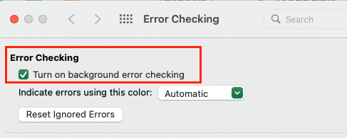
- Select the “Enable background error checking” checkbox.
- Check or uncheck boxes for the error types you want to include/exclude.
- Click “OK” to apply the filter.
Now, as you navigate with the “Next” and “Previous” buttons, Excel will only stop on the selected error types.
Customize Error Checking Rules in Excel
Excel lets you fine-tune the rules it uses to identify potential errors, giving you more control over the error checking process.
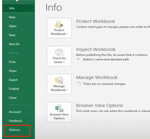
Accessing Formula Options
- Click the “File” tab and select “Options” at the bottom of the menu.

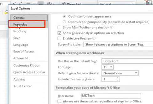
- In the Excel Options dialog, select “Formulas” from the left sidebar.

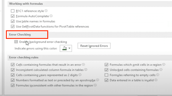
- Scroll down to the “Error checking” section to view available options.

Here you can enable or disable background error checking, change error indicator colors, and select which error rules to apply.
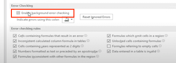
Selecting Specific Rules to Enable/Disable
In the “Error checking rules” section, you’ll see a list of available rules, each with a checkbox. These include:
- Cells containing formulas that result in an error
- Inconsistent calculated column formula in tables
- Cells containing years represented as 2 digits
- Numbers formatted as text or preceded by an apostrophe
- Formulas inconsistent with other formulas in the region
- Formulas which omit cells in a region
- Unlocked cells containing formulas
Check or uncheck boxes to enable or disable specific rules based on your needs.
Choosing Error Indicator Colors
Excel uses green triangle indicators by default to flag potential errors in cells. However, you can choose a different color if desired:
- In the “Indicate errors using” dropdown, select the color you prefer.
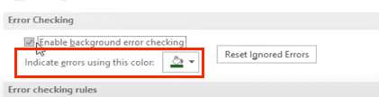
- Click “OK” to apply the change.
Now cells with errors will display your chosen indicator color.

Stop exporting data manually. Sync data from your business systems into Google Sheets or Excel with Coefficient and set it on a refresh schedule.
Get Started
Remove Green Triangle Error Indicators
If you find the green triangle error indicators more distracting than helpful, you can turn them off. Here’s how:
Turning Off Background Error Checking
- Click the “File” tab and select “Options.“
- Go to the “Formulas” category in the Excel Options dialog.
- Under “Error checking“, uncheck the “Enable background error checking” box.
- Click “OK” to apply the change.
With background error checking disabled, cells will no longer display green triangle indicators, even if they contain potential errors.
Disabling Specific Error Types
If you only want to disable certain types of error indicators:
- In Excel Options > Formulas, click the “Error Checking Options” button under “Error Checking“.
- Uncheck the boxes for any error types you want to exclude from background checking.
- Click “OK” to close the dialog, then “OK” again to apply changes.
Excel will now skip those error types when analyzing your spreadsheet.
Temporary vs. Permanent Indicator Removal
Unchecking “Enable background error checking” turns off error indicators for all spreadsheets. However, this setting is workbook-specific.
To temporarily hide error indicators for the current session only:
- Press Alt+F8 to open the Error Checking dialog if any errors are present.
- Click “Options” and uncheck “Enable background error checking“.
- Click “OK” to dismiss the dialog.
Indicators will reappear the next time you open the workbook unless you save it with background checking turned off.
Common Excel Errors and Their Solutions
Knowing how to interpret and resolve the most common Excel errors is key to keeping your spreadsheets running smoothly. Let’s look at fixes for three frequent offenders:
#DIV/0! Error Resolution
The #DIV/0! error occurs when a formula attempts to divide by zero or an empty cell. To resolve it:
- Check the divisor (denominator) in your formula for 0 or null values.
- If dividing by a cell reference, ensure the referenced cell contains a non-zero value.
- To handle potential divide-by-zero errors gracefully, use the IFERROR function: =IFERROR(numerator/denominator, “Error message”)
This will return your specified error message text instead of #DIV/0! when a divide-by-zero occurs.
#NAME? Error Fixes
The #NAME? error appears when Excel doesn’t recognize text in a formula, often due to misspelled function names or range names. Here’s how to fix it:
- Double-check spelling of functions and named ranges in the formula.
- Verify that any named ranges used actually exist in the workbook.
- Ensure there are no errant quotes or punctuation throwing off syntax.
- Rebuild the formula using the Insert Function dialog (Shift+F3) to ensure proper syntax.
Carefully proofreading formulas will prevent most #NAME? errors.
#REF! Error Handling
The #REF! error indicates an invalid cell reference, often caused by deleting rows/columns that formulas refer to. To resolve:
- Note the cell(s) with #REF! errors.
- Select each errored cell and view its formula in the formula bar.
- Identify the invalid reference (often “####REF!”) and update it to a valid range.
- Consider using named ranges or table references to make formulas more resilient to insertions/deletions.
Regularly auditing and updating formulas will minimize #REF! errors in your spreadsheets.
Use Formula Auditing Tools
Excel’s Formula Auditing tools are invaluable for tracking down the source of stubborn formula errors. Here’s how to leverage them:
Tracing Precedents and Dependents
To visually trace relationships between formula cells and the cells they reference or are referenced by:
- Select a cell containing a formula.
- On the Formulas tab, click “Trace Precedents” to see which cells feed data into the selected cell.
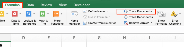
- Click “Trace Dependents” to see which cells rely on the selected cell in their formulas.

- Continue clicking the Precedents or Dependents button to trace relationships across multiple levels.
- Click “Remove Arrows” to clear the tracer arrows from your spreadsheet.
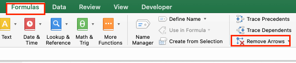
This is incredibly helpful for understanding how data flows through your formulas.
Evaluating Complex Formulas
For formulas with lots of nested functions, the Formula Evaluation tool helps break them down into digestible steps:
- Select a cell with a complex formula you want to analyze.
- Click the “Evaluate Formula” button in the Formula Auditing group.

- In the Evaluate Formula dialog, click “Evaluate” to see the formula’s innermost function resolve to a value.

- Continue clicking “Evaluate” to work through each function in the formula.
- When finished, click “Close” to dismiss the dialog.
Slowly stepping through a formula’s logic can clarify what’s happening and reveal errors.
Next Steps
Regularly applying these error checking methods to your spreadsheets will help ensure they remain accurate, reliable, and error-free. Make spreadsheet auditing a habitual practice to catch and correct small problems before they blossom into major headaches.
Now that you’ve mastered the core error checking workflow, consider exploring advanced formula auditing with Coefficient. Their suite of tools builds on Excel’s functionality, helping you understand and optimize your spreadsheets in greater depth. Visit their site to learn more and start a free trial.


