Excel’s conditional formatting helps you spot trends and patterns in your data by automatically changing how cells look based on rules you set. Whether you need to highlight sales targets, flag overdue tasks, or mark duplicate entries, conditional formatting makes it simple to spot what matters in your spreadsheets.

How to Apply Basic Conditional Formatting in Excel

Let’s start with the essential steps to format cells based on their contents:

1. Select your target cells
   Click and drag to highlight the range you want to format
2. Find conditional formatting options
   
   
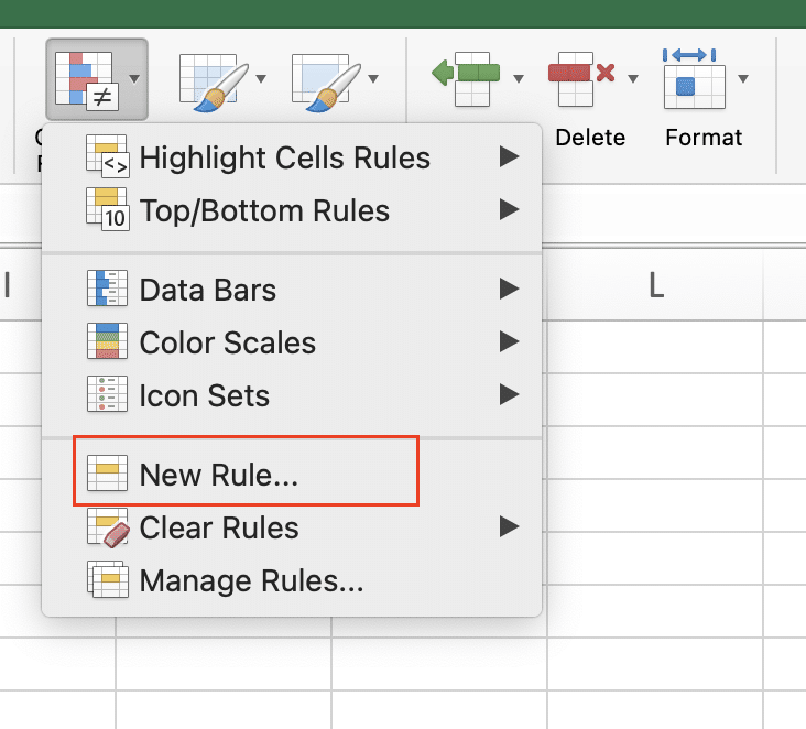
   Click Home > Conditional Formatting in the Styles group

1. Pick a rule type
   Choose from Highlight Cell Rules, Top/Bottom Rules, Data Bars, Color Scales, or Icon Sets

1. Set your conditions
   
   
   Enter values, choose colors, and adjust formatting options in the dialog box

Creating Color-Based Cell Rules

Color rules help you quickly spot values that meet specific criteria:

Rule Type	Example	Use Case
Greater Than	>1000 = Red	Sales above target
Less Than	<0 = Yellow	Negative balances
Between	50-100 = Green	Acceptable ranges
Duplicate Values	Duplicate = Orange	Find repeated entries

To set up a basic color rule:

1. Select your data range

2. Click Home > Conditional Formatting > Highlight Cell Rules

3. Choose a comparison type (greater than, less than, between, etc.)

4. Enter your values

5. Select your formatting style

Using Text-Based Formatting Rules

Text rules let you format cells based on their content:

Text Condition	Format Example	Common Use
Contains	“Urgent” = Red	Priority items
Starts With	“Q1” = Blue	Quarterly data
Ends With	“Draft” = Gray	Document status

To create a text-based rule:

1. Select your range

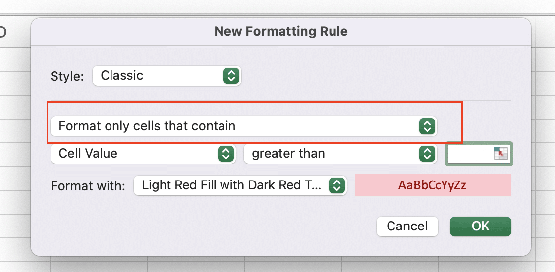
2. Click Conditional Formatting > New Rule

3. Choose “Format only cells that contain”

4. Select “Specific Text” from the dropdown

5. Enter your text criteria

Working with Formulas in Conditional Formatting

Custom formulas give you precise control over your formatting rules:

Example formula rule:

=$B2>$C2

This formats cells where column B values exceed column C values.

Tips for formula-based formatting:

• Use absolute references ($) for column letters when needed
• Start formulas with = sign
• Test your formula on a small range first

IF Statement Examples for Formatting

Here’s how to use IF statements in your conditional formatting:

Purpose	Formula Example	Result
Compare Columns	=IF($B2>$C2,TRUE,FALSE)	Highlights when B>C
Multiple Conditions	=AND($B2>0,$C2<100)	Both conditions must be true
Either/Or	=OR($B2=”Yes”,$C2=”No”)	Either condition can be true

Creating Multi-Condition Format Rules

To manage multiple rules:

Set rule order


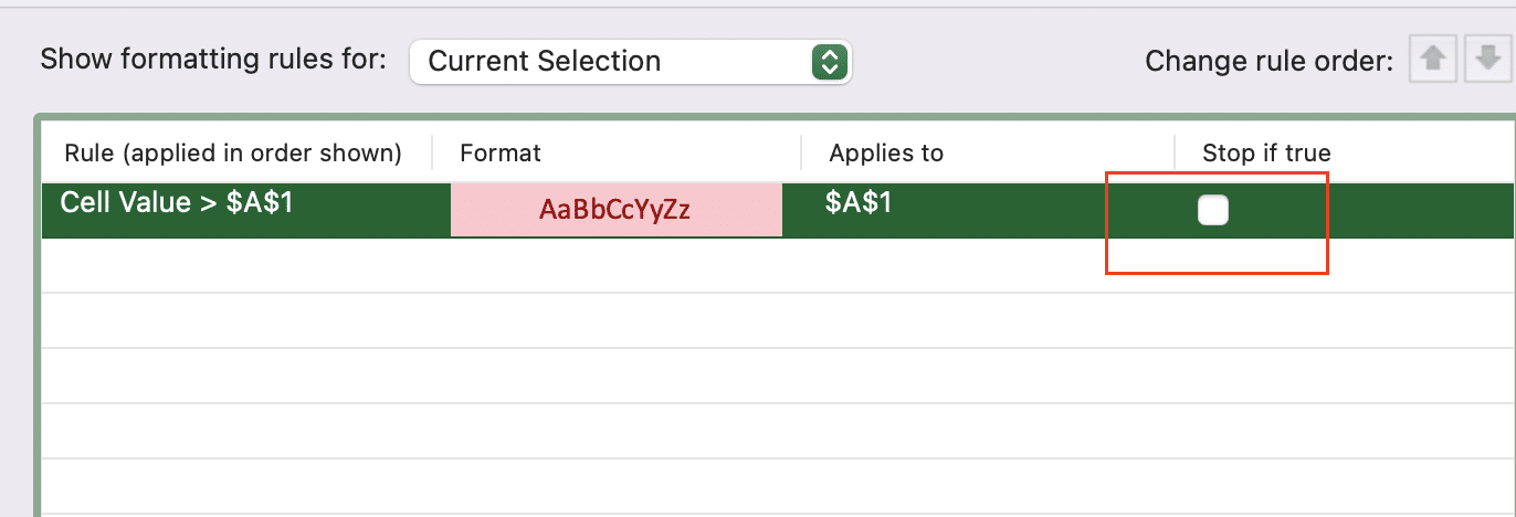
Open Conditional Formatting > Manage Rules

1. Use arrows to arrange rules by priority

Combine rules

Apply multiple rules to the same range

1. Check “Stop if True” for exclusive rules

Icon Sets and Visual Indicators

Icon sets add visual markers to your data:

Icon Type	Best For	Setup Steps
Arrows	Trends	Select range > Conditional Formatting > Icon Sets
Traffic Lights	Status	Choose 3-symbol set for Red/Yellow/Green
Ratings	Rankings	Pick 4-5 symbols for detailed grading

What You Can Do Next

Review your formatting rules regularly to ensure they still match your needs. Save your favorite formatting combinations as templates for future use.

Want to keep your conditional formatting rules updated with live data? Try Coefficient to connect your spreadsheets directly to your business systems. Get started with Coefficient and ensure your Excel formatting always reflects your latest data.