What Is The CHOOSE Function?
The Excel CHOOSE function allows one to choose a value from a list based on a given index number. It helps in decision-making in spreadsheets by enabling the user to access specific data points on demand. The CHOOSE function can be helpful to users who have to deal with large amounts of data and have difficulty finding the necessary information. This function is especially useful in data analysis for scenario analysis or data validation because it offers a flexible and fast way to access data.
The readers can expect to read about how to use the CHOOSE function and how it can help them in better data management and analysis in the coming content.
Understanding The CHOOSE Function
The CHOOSE function in Excel selects a value from a list of values based on a specified position index. This function is especially useful in scenarios where a decision needs to be made among multiple possibilities. The syntax for the CHOOSE function is as follows:
=CHOOSE(index_num, value1, [value2], …)
The components of the CHOOSE Function are:
- index_num: The position of the value to return, based on the list provided. The index_num must be a number.
- value1, value2, …: These are the list of values from which the function chooses. The number of values can vary, but index_num should be within the range of values listed.
Example Formula:
=CHOOSE(3, “Apple”, “Banana”, “Cherry”, “Date”)
In this formula:
- The index_num is 3.
- The CHOOSE function looks at the third position in the list provided, which is “Cherry”.
- Therefore, the function returns “Cherry”.
Important Notes:
The index_num must be an integer between 1 and the number of choices provided. If index_num is less than 1 or greater than the number of values listed, CHOOSE will return a #VALUE! error.
CHOOSE can be used to simplify decision-making in your spreadsheets by selecting data based on its position in a given list.
It can also be combined with other functions to enhance its utility, such as using it within IF statements or alongside VLOOKUP for dynamic decision flows.
How Does CHOOSE Function Work In Excel?
The CHOOSE function in Excel is a powerful tool that simplifies the selection of specific items based on a given index number. It’s particularly useful for scenarios where you need to pick one out of several possible outcomes. Below, we break down how to effectively use the CHOOSE function in Excel, complete with a step-by-step guide and a sample dataset.
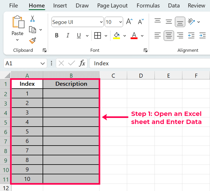
Step 1: Open An Excel Sheet And Enter Data
Start by opening Excel and either create a worksheet where you want to use the CHOOSE function. Input or identify the data you will work with using the CHOOSE function. This is where you define the parameters that will be used to select your outcome.
Here’s a simple dataset with 10 rows that we’ll use to demonstrate the CHOOSE function:

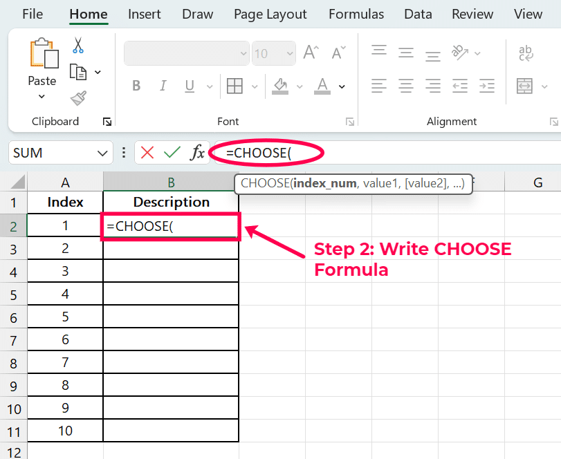
Step 2: Write CHOOSE Formula
Click on the cell where you want the CHOOSE function’s result to be displayed. Then, type the formula starting with ‘=CHOOSE(‘.

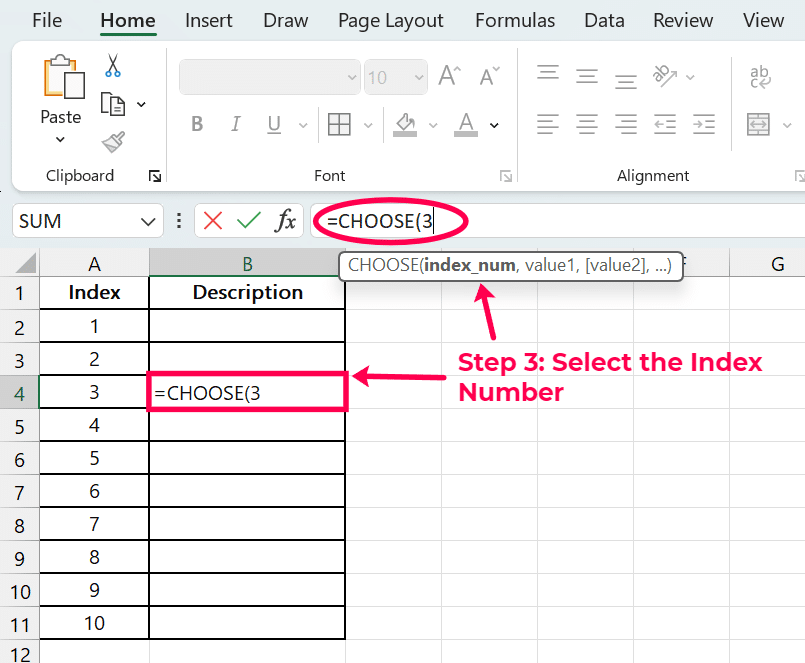
Step 3: Select The Index Number
Decide the index_num which corresponds to the item you want to select. This is usually based on a logical condition or specific scenario in your dataset. Then, put the index_num as the first argument inside the CHOOSE function. This number determines which value or reference is selected.

Step 4: Add Possible Outcomes
Following the index_num, list down the values or cell references from which the CHOOSE function will select. These could be direct inputs like “Apple”, “Banana”, “Cherry”, etc., or references to cells containing these values.

Step 5: Complete The Formula
Finish the formula with the parenthesis ‘)’. Hit the Enter key to execute the formula and display the result.

In this example, the index number 3 selects “Cherry” from the list of values provided. When you press Enter, “Cherry” will be displayed in the cell where you entered the formula.
Video Tutorial
Check out the tutorial below for a complete video walkthrough!
Examples Of CHOOSE Function In Use
Example 1: Basic Selection
Here, it will choose the month based on its number. Formula:
=CHOOSE(2, “January”, “February”, “March”)
The CHOOSE function in Excel selects a value from a list of values based on a given index number. In this example, the index number is 2. The function looks at the list of months provided (“January”, “February”, “March”) and returns the second item in the list, which is “February”.

Example 2: Nested CHOOSE With Other Functions
Consider a case where a school teacher wishes to use Excel to compare the performance of students in various subjects. The teacher wants to calculate either the total or the average score based on a selected option. This can be easily achieved using the CHOOSE function in conjunction with SUM and AVERAGE.
Our dataset consists of 10 rows, representing scores of 10 students in three subjects: Mathematics, Science, and English.
The formula should allow the user to input a number (1 for total scores, 2 for average scores). Use the CHOOSE function to select the appropriate calculation based on the input. Suppose cell F2 contains the user’s choice (1 or 2). The formula in G2 would look like this:

Stop exporting data manually. Sync data from your business systems into Google Sheets or Excel with Coefficient and set it on a refresh schedule.
Get Started
=CHOOSE(F2, SUM(B2:D2), AVERAGE(B2:D2))
This formula checks the value in F2. If it is 1, it calculates the sum of the scores from columns B to D for the first student. If it is 2, it calculates the average.

Common Errors In CHOOSE Function
The CHOOSE function in Excel is a good formula that helps you to pick one value from a list of values using an index number. But there are several common errors that users face when using this function. Here’s a detailed breakdown:
Incorrect Index Number
The CHOOSE function expects the index number to be a valid reference; if the index number is less than 1 or greater than the number of values provided, Excel will return #VALUE! error.
Users have to make sure that the index number is correct according to the length of the list. For example =CHOOSE(0, “A”, “B”, “C”) returns an error because there is no zeroth option.
Non-integer Index Number
If the index number is not an integer, Excel will round it down to the integer part. For example, CHOOSE(2. 9, “A”, “B”, “C”) will return “B”. This can lead to unpredictable results if the user inputs a decimal value by mistake.
Using Non-numeric Index
The index argument must be numeric. It will return #VALUE! error if a non-numeric value or a text string that cannot be converted to a number is used.
Array Limitation
The CHOOSE function can only accept up to 254 value arguments. If more than 254 values are attempted to be included then a #VALUE! error will occur.
These points are essential for the correct use of the CHOOSE function and the most common mistakes that can affect the work with data in Excel.
Tips and Tricks
Optimize the Use of CHOOSE with Large Data Sets
- Limit Choices – It is important to note that CHOOSE can accept multiple inputs but it is recommended to limit the number of choices to avoid complex and difficult-to-read formulas. This is especially important when dealing with large data sets to avoid confusion.
- Use With Array Formulas – If you are dealing with large arrays, use CHOOSE in conjunction with array formulas to process several data sets simultaneously.
- Pre-Calculate Values – If you can, try to calculate or simplify expressions before passing them to CHOOSE. This makes the function computation faster especially when the data is large.
- Integration with LOOKUP Functions – For large data sets, it is recommended to use CHOOSE in conjunction with other lookup functions such as VLOOKUP or INDEX/MATCH to manage data more efficiently and save time.
- Memory Management – Remember to keep an eye on the memory usage in Excel when working with large data sets. Organizing your CHOOSE function and its related formulas in a more efficient manner will also help you save memory and avoid slowdowns.
Using The CHOOSE Function In Excel
Now that we’ve discussed how to use the CHOOSE function in Excel to speed up and simplify data analysis, you can be even more efficient in your day to day tasks.
Unlock even more efficiency with Coefficient and take your business to the next level! This reliable platform facilitates the transfer of live data from various sources to Google Sheets and Excel in an automated manner, eliminating the need for manual data transfers.
Coefficient makes it possible for your team to work with the latest data at all times, enables real-time decision-making, and improves efficiency by eliminating the need for manual data transfers. Some of the benefits of the new features include automatic refreshes, direct updates, and real-time alerts, which help to make your operations more efficient. Are you ready to change the way you manage data? Sign up for a free trial today and see how connected spreadsheets can transform your business!


