How to Average Time in Excel: A Comprehensive Guide

Are you struggling to calculate average times in Excel?

Whether you’re tracking project durations, analyzing customer service response times, or managing employee work hours, knowing how to average time data is crucial for effective analysis and decision-making.

This guide will walk you through everything you need to know about averaging time in Excel, from basic techniques to advanced methods for handling complex scenarios.

Understanding Time Formats in Excel

Before we dive into averaging time, it’s crucial to understand how Excel handles time data.

Excel’s Time Data Type

Excel stores time as a decimal fraction of a 24-hour day. For example:

• 12:00 PM is stored as 0.5 (half a day)
• 6:00 AM is stored as 0.25 (quarter of a day)
• 6:00 PM is stored as 0.75 (three-quarters of a day)

This system allows Excel to perform calculations on time values easily. However, it also means that you need to be careful about how you input and format time data to ensure accurate results.

Common time formats in Excel include:

• hh:mm AM/PM (e.g., 02:30 PM)
• hh:mm:ss (e.g., 14:30:00)

To input time data correctly, use a colon (:) to separate hours, minutes, and seconds. Excel will automatically recognize this as a time value.

Formatting Cells for Time Calculations

Proper cell formatting is essential for accurate time calculations. Here’s how to format cells for time data:

1. Select the cells containing time data
2. Right-click and choose “Format Cells“

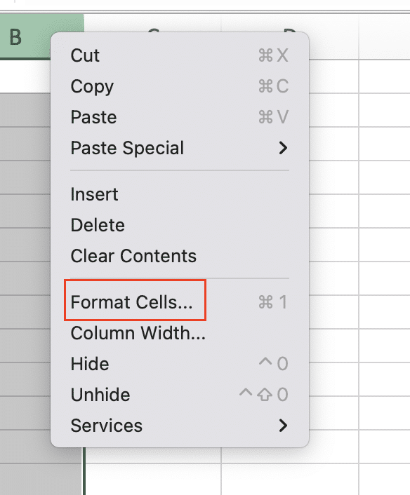
1. In the “Number” tab, select “Time” from the Category list

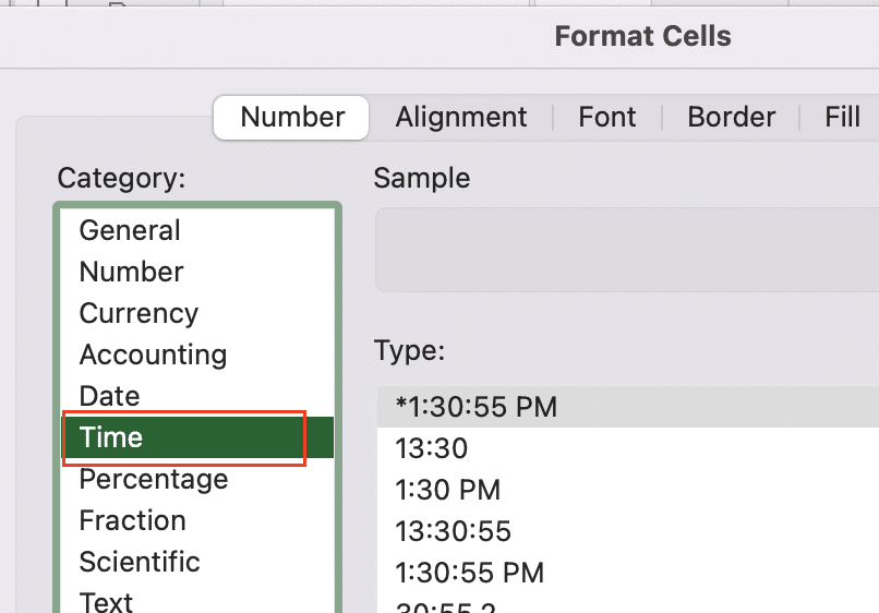
1. Choose the desired time format from the Type list

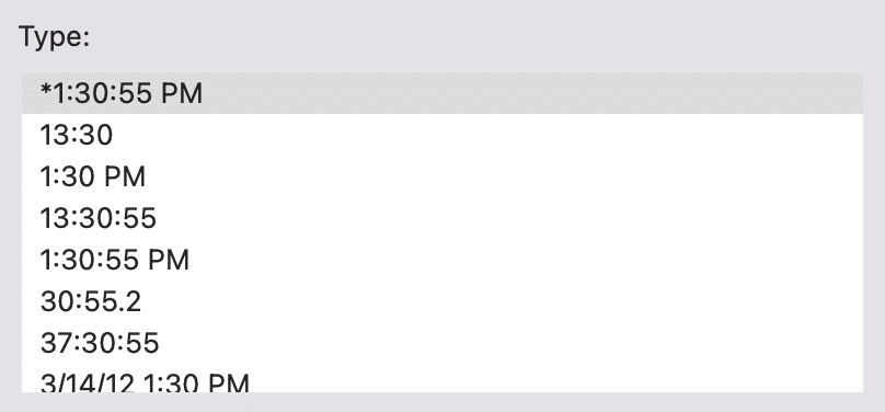
1. Click “OK” to apply the formatting.

For custom time formats, you can use the following codes:

• h or hh: Hours
• m or mm: Minutes
• s or ss: Seconds
• AM/PM: 12-hour clock indicator

For example, a custom format of “hh:mm:ss” would display time as 13:45:30.

If you encounter issues with time calculations, check your cell formatting first. Incorrect formatting is a common source of errors when working with time data in Excel.

Using the AVERAGE Function for Time Calculations

The AVERAGE function is the most straightforward way to calculate the average time in Excel. Let’s explore how to use it effectively.

Basic AVERAGE Function Syntax

The syntax for the AVERAGE function is:

=AVERAGE(number1, [number2], …)

Where “number1” is the first number or cell reference, and subsequent arguments are optional.

To use AVERAGE with time data:

1. Enter your time values in separate cells
2. In a new cell, type =AVERAGE(

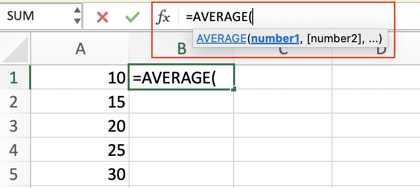
1. Select the range of cells containing your time values
2. Close the parenthesis and press Enter

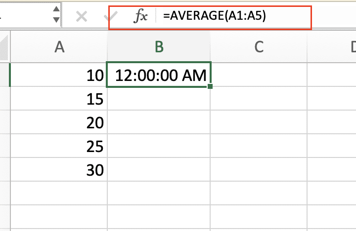
Example: If you have time values in cells A1:A5, your formula would be:

=AVERAGE(A1:A5)

Advanced AVERAGE Function Techniques

For more complex time averaging scenarios, consider these advanced techniques:

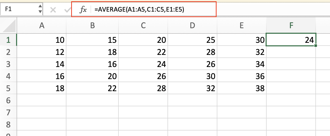
1. Using AVERAGE with cell ranges: You can average times across multiple columns or non-contiguous ranges:
   
   =AVERAGE(A1:A5,C1:C5,E1:E5)

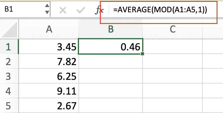
1. Handling mixed data types: If your data includes both dates and times, use the MOD function to extract only the time portion:
   
   =AVERAGE(MOD(A1:A5,1))

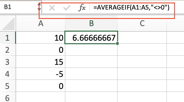
1. Excluding blank cells or zero values: Use AVERAGEIF to ignore empty cells or cells with zero time values:
   
   =AVERAGEIF(A1:A5,”<>0″)

Remember to format the result cell as a time value to display the average correctly.

Alternative Methods for Averaging Time

While the AVERAGE function works well for simple scenarios, you may need more advanced methods for complex time averaging tasks.

Using SUMPRODUCT for Weighted Time Averages

The SUMPRODUCT function allows you to calculate weighted time averages, which is useful when certain time values should have more influence on the result than others.

Syntax:

=SUMPRODUCT(time_range, weight_range) / SUM(weight_range)

Example scenario: Let’s say you’re calculating the average response time for customer service tickets, but you want to give more weight to recent tickets.

1. Enter your time data in column A
2. Enter weights in column B (higher numbers for more recent tickets)
3. Use the following formula:
   
   =SUMPRODUCT(A1:A10,B1:B10) / SUM(B1:B10)

1. Format the result cell as a time value

This formula will give you a weighted average of the response times, with recent tickets having a greater influence on the result.

Leveraging AVERAGEIFS for Conditional Time Averaging

The AVERAGEIFS function allows you to calculate average times based on multiple criteria.

Syntax:

=AVERAGEIFS(average_range, criteria_range1, criteria1, [criteria_range2, criteria2, …])

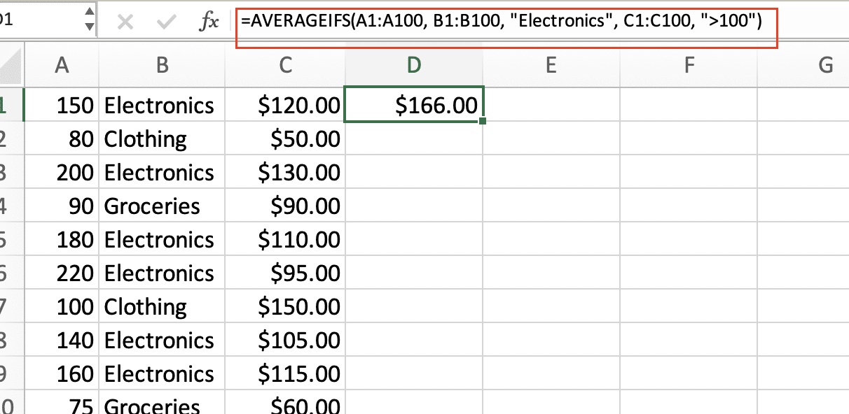
Real-world example: Suppose you want to calculate the average processing time for orders, but only for a specific product category and orders over $100.

1. Enter order processing times in column A
2. Enter product categories in column B
3. Enter order amounts in column C
4. Use the following formula:
   
   =AVERAGEIFS(A1:A100, B1:B100, “Electronics”, C1:C100, “>100”)

1. Format the result cell as a time value

This formula will average the processing times only for orders in the “Electronics” category with an order amount greater than $100.

Handling Special Cases in Time Averaging

Time calculations can become tricky in certain scenarios. Let’s address two common special cases.

Averaging Time Across Midnight

When averaging times that span midnight, a simple AVERAGE function may produce incorrect results. To solve this, use the following approach:

1. Calculate the time difference from midnight for each value
2. Average these differences
3. Add the result back to midnight

Here’s a formula that accomplishes this:

=TIME(0,0,0) + AVERAGE(MOD(A1:A5-TIME(0,0,0)+1,1))

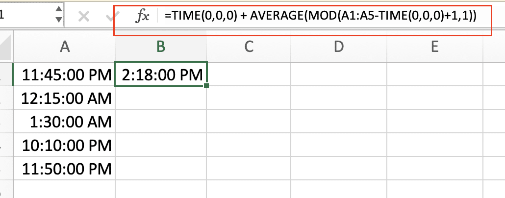
This formula works by:

• Subtracting midnight (TIME(0,0,0)) from each time value
• Adding 1 to ensure positive values
• Using MOD to get the fractional part of a day
• Averaging these fractions
• Adding the result back to midnight

Example: If you have times like 23:30, 00:30, 01:30 in cells A1:A3, this formula will correctly calculate their average.

Calculating Average Duration

When working with time durations (e.g., task completion times), you may need to handle values exceeding 24 hours. Here’s how to average durations:

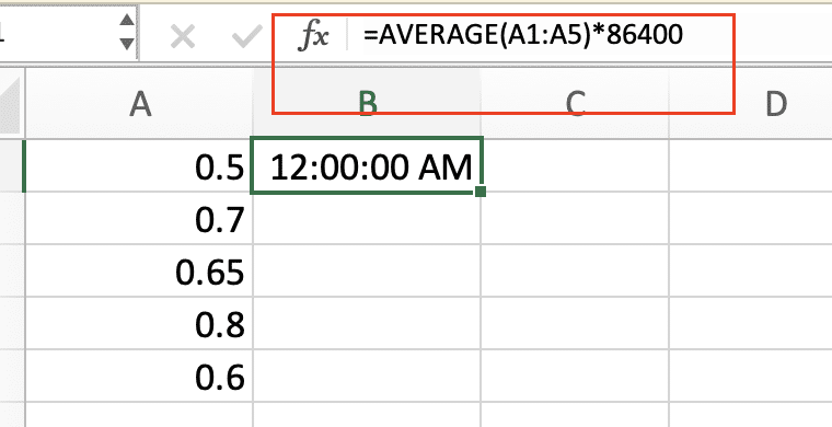
1. Enter durations in a h:mm:ss format
2. Use this formula to calculate the average in seconds:
   
   =AVERAGE(A1:A5)*86400

1. Convert the result back to a duration format:
   
   =TEXT(AVERAGE(A1:A5),”[h]:mm:ss”)

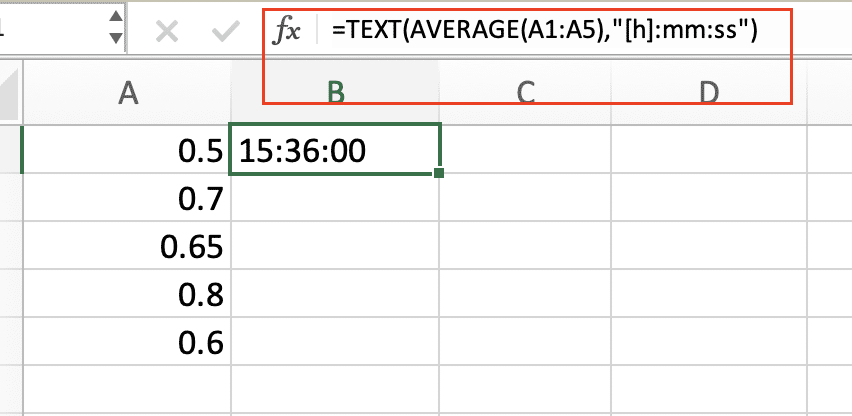
This approach allows you to accurately average durations that may exceed 24 hours.

Visualizing Time Averages in Excel

After calculating time averages, visualizing the data can provide valuable insights.

Creating Charts for Time Data

To create a chart for time-based data:

1. Select your time data range
2. Go to the Insert tab and choose an appropriate chart type (e.g., Column or Line)

1. Right-click on the horizontal axis and select “Format Axis“

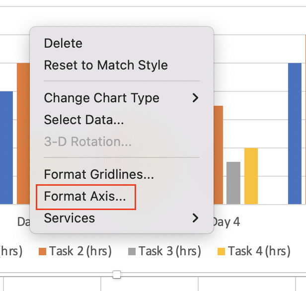
1. In the “Axis Options,” set the “Number” to “Time“

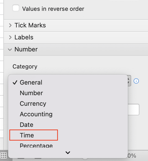
1. Adjust the “Base unit” and “Major unit” as needed (e.g., Days, Hours, Minutes)

For comparing actual times to average times:

1. Calculate your average time
2. Create a new column with this average repeated for each data point
3. Create a combo chart with columns for actual times and a line for the average

Using Conditional Formatting with Time Averages

Conditional formatting can help highlight time values above or below the average:

1. Select your time data range
2. Go to Home > Conditional Formatting > New Rule

1. Choose “Use a formula to determine which cells to format“
2. Enter a formula like: =A1>AVERAGE($A$1:$A$10)
3. Click “Format” and choose a color or style
4. Repeat for below-average values with <AVERAGE($A$1:$A$10)

This will automatically highlight values above and below the average, making it easy to spot trends or outliers in your time data.

Average Time in Excel

Mastering time averaging in Excel opens up a world of possibilities for data analysis and reporting. We’ve covered various methods, from basic AVERAGE functions to advanced techniques like weighted averages and conditional averaging. Remember to always pay attention to your data formats and use the appropriate method for your specific scenario.

Practice these techniques with your own data to become proficient in time calculations. As you gain confidence, you’ll find that Excel becomes an even more powerful tool for time-based analysis in your work.

Ready to take your Excel data analysis to the next level? Get started with Coefficient (https://coefficient.io/get-started) to enhance your spreadsheet capabilities and streamline your data workflows. With Coefficient, you can easily import, refresh, and analyze data from various sources, making your time calculations even more powerful and insightful.