Got negative numbers in your spreadsheet that need to become zeros? Whether you’re cleaning financial data or preparing reports, converting negative values to zero is a common task. Let’s explore multiple ways to handle this in both Excel and Google Sheets.

Using the MAX Function: The Simplest Solution

The MAX function offers a straightforward way to convert negative numbers to zero. It compares your cell value with zero and returns the larger number.

Basic MAX Function Implementation

Command: Create a basic MAX formula

1. Select the cell where you want the converted value
2. Type the formula: =MAX(0,A1)

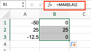
1. Press Enter
2. The formula returns zero for negative numbers and keeps positive numbers unchanged

Here’s how the MAX function handles different values:

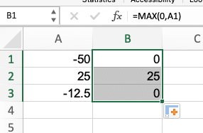
Applying MAX to Multiple Cells

Command: Copy the MAX formula across ranges

1. Enter the formula in your first cell
2. Click the small square in the bottom-right corner
3. Drag across your desired range
4. Release to apply the formula

Pro tip: Double-click the fill handle to automatically copy the formula down to match your data range.

IF Statements: More Control Over Your Conversions

IF statements provide additional flexibility when converting negative numbers. They’re especially useful when you need to add conditions beyond simple conversion.

Command: Create an IF statement for conversion

1. Select your target cell
2. Enter: =IF(A1<0,0,A1)

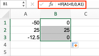
1. Press Enter

This formula reads: If the value in A1 is less than zero, return zero; otherwise, return the original value.

Example implementations:

Scenario	Formula	Description
Basic conversion	=IF(A1<0,0,A1)	Converts negatives to zero
With rounding Try the Free Spreadsheet Extension Over 500,000 Pros Are Raving About Stop exporting data manually. Sync data from your business systems into Google Sheets or Excel with Coefficient and set it on a refresh schedule. Get Started	=IF(ROUND(A1,2)<0,0,A1)	Rounds to 2 decimals before converting
Multiple conditions	=IF(AND(A1<0,A1>-100),0,A1)	Only converts numbers between -100 and 0

Converting Negative Numbers in Google Sheets

Google Sheets handles these conversions similarly to Excel, with slight syntax differences.

Command: Apply conversions in Google Sheets

1. Use =MAX(0,A1) for simple conversions
2. For array formulas, add ARRAYFORMULA: =ARRAYFORMULA(MAX(0,A1:A100))

Working with Large Datasets

When handling extensive data:

Command: Optimize large dataset conversion

1. Copy your data to a new column
2. Use Find and Replace for permanent changes:
   • Press Ctrl+H (Cmd+H on Mac)

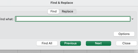
• • In “Find” enter: -[0-9]*
  • In “Replace with” enter: 0

1. Check “Match using regular expressions“

Formula-Free Methods

Sometimes, you need quick, permanent changes without formulas.

Command: Use Paste Special for permanent conversion

1. Copy your range
2. Right-click > Paste Special > Values

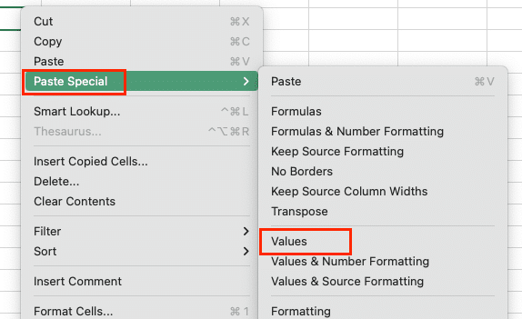
1. Apply Find and Replace

1. Choose “Match entire cell contents“

Preserving Original Data

Always protect your source data:

Command: Create a backup before converting

1. Right-click column header
2. Select “Insert 1 column left“
3. Copy original data to new column
4. Hide the backup column if needed

Next Steps: Choose the method that best fits your needs.

For simple conversions, MAX works great. For complex conditions, use IF statements. Remember to back up your data before making permanent changes.

Want to automate your spreadsheet workflows and keep your data in sync? Try Coefficient to connect your business systems directly to your spreadsheets. Get started with Coefficient and eliminate manual data updates.