Excel is a crucial tool for accounting and finance professionals. This guide covers the top 10 Excel formulas that can significantly improve your work efficiency and accuracy. Each section includes detailed explanations, practical examples, and tips for effective use.

1. VLOOKUP: Retrieving Data from Large Datasets

VLOOKUP helps you find and pull specific information from large datasets. It’s particularly useful for tasks like populating invoice details or finding customer information.

How to Use VLOOKUP

The basic syntax is:

=VLOOKUP(lookup_value, table_array, col_index_num, [range_lookup])

• lookup_value: The value you’re searching for
• table_array: The range of cells containing your data
• col_index_num: The column number in the range containing the return value
• range_lookup: TRUE for approximate match, FALSE for exact match (always use FALSE for accounting purposes)

Practical Example

Imagine you have a customer database and need to find a customer’s outstanding balance:

Customer ID	Customer Name	Credit Limit	Outstanding Balance
C001	Acme Corp	$50,000	$15,000
C002	Beta Industries	$75,000	$30,000
C003	Gamma Services	$100,000	$45,000

To find the outstanding balance for customer C002:

excel

Copy

=VLOOKUP(“C002”, A1:D4, 4, FALSE)

This formula will return $30,000.

Tips for Effective Use

1. Always use FALSE as the last argument for exact matches in financial data.
2. Ensure your lookup value is in the leftmost column of your table array.
3. If you’re working with large datasets, consider using INDEX MATCH instead for better performance.

2. SUMIFS: Conditional Summing for Complex Criteria

SUMIFS allows you to sum values that meet multiple criteria. It’s essential for creating summary reports and analyzing data across various categories.

How to Use SUMIFS

The syntax is:

=SUMIFS(sum_range, criteria_range1, criteria1, [criteria_range2, criteria2, …])

• sum_range: The range of cells you want to sum
• criteria_range1: The range that should be tested against criteria1
• criteria1: The condition that must be met

Practical Example

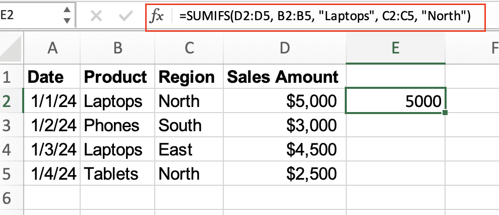
Consider a sales dataset:

Date	Product	Region	Sales Amount
1/1/2024	Laptops	North	$5,000
1/2/2024	Phones	South	$3,000
1/3/2024	Laptops	East	$4,500
1/4/2024	Tablets	North	$2,500

To sum all laptop sales in the North region:

=SUMIFS(D2:D5, B2:B5, “Laptops”, C2:C5, “North”)

This formula will return $5,000.

Tips for Effective Use

1. You can add multiple criteria pairs to create complex conditions.
2. Use wildcards (*) in text criteria for partial matches.
3. For date ranges, use comparison operators like “>1/1/2024” to specify periods.

3. EOMONTH and EDATE: Precision in Financial Period Calculations

EOMONTH and EDATE are crucial for handling date-based calculations in financial reporting and forecasting.

How to Use EOMONTH and EDATE

EOMONTH syntax:

excel

Copy

=EOMONTH(start_date, months)

EDATE syntax:

=EDATE(start_date, months)

• start_date: The initial date you’re working with
• months: The number of months to move forward (positive) or backward (negative)

Practical Examples

1. To find the last day of the current month:
   
   =EOMONTH(TODAY(),0)
2. To calculate the date for a quarterly report three months from now:
   =EDATE(TODAY(),3)
3. To find the last day of the previous month:
   
   =EOMONTH(TODAY(),-1)

Tips for Effective Use

1. Combine EOMONTH with the DATE function to create specific end-of-month dates.
2. Use EDATE for rolling date calculations in financial models.
3. Remember that EOMONTH always returns the last day of a month, while EDATE preserves the day of the month.

4. Nested IF Statements: Building Complex Logical Structures

Nested IF statements allow you to create complex decision trees within your spreadsheets, crucial for categorization and conditional analysis.

How to Use Nested IF Statements

The basic structure is:

=IF(condition1, value_if_true1, IF(condition2, value_if_true2, value_if_false))

Practical Example

Let’s categorize accounts receivable based on days outstanding:

Invoice Date	Days Outstanding	Category
1/1/2024	30	Current
12/1/2023	61	31-60 Days
11/1/2023	91	Over 90 Days

Formula for categorization:

 

=IF(B2>90,”Over 90 Days”,IF(B2>60,”61-90 Days”,IF(B2>30,”31-60 Days”,”Current”)))

Tips for Effective Use

1. Start with the most extreme condition and work your way back.
2. Limit nesting to 3-4 levels for readability; consider using IFS function in newer Excel versions for more complex logic.
3. Use AND/OR functions within IF statements for multiple conditions.

5. ROUND: Ensuring Consistency in Financial Figures

ROUND is essential for maintaining precision and consistency in financial calculations and reporting.

How to Use ROUND

The syntax is:

=ROUND(number, num_digits)

• number: The value you want to round
• num_digits: The number of decimal places to round to (use negative numbers to round to tens, hundreds, etc.)

Practical Example

Rounding calculated ratios or percentages:

Gross Profit	Revenue	Gross Margin (Raw)	Gross Margin (Rounded)
$256,789.45	$1,000,000.00	0.25678945	0.2568

Formula:

excel

Copy

=ROUND(A2/B2,4)

This rounds the gross margin to four decimal places, resulting in 0.2568 or 25.68%.

Tips for Effective Use

1. Use ROUNDUP or ROUNDDOWN for specific scenarios where you always need to round in a particular direction.
2. Be consistent with rounding across all financial statements to ensure accuracy.
3. Consider materiality when deciding on the number of decimal places to use.

6. AGGREGATE: Advanced Calculations for Financial Analysis

AGGREGATE is a powerful function that combines the functionality of several other functions, making it ideal for complex financial analysis.

How to Use AGGREGATE

The syntax is:

excel

Copy

=AGGREGATE(function_num, options, array, [k])

• function_num: A number 1-19 specifying which function to use (e.g., 1 for AVERAGE, 4 for MAX)
• options: A number specifying which data to ignore (e.g., 6 to ignore errors and hidden rows)
• array: The range of cells to perform the function on
• [k]: Optional, used with certain function numbers

Practical Example

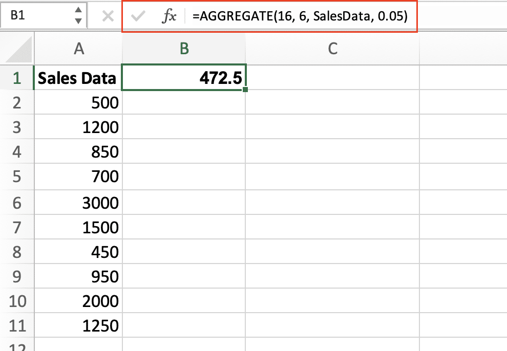
Calculate the average sales, ignoring the top 5% of values and any errors:

excel

Copy

=AGGREGATE(1, 6, SalesData, 0.05)

This formula calculates the average (function 1) of the SalesData range, ignoring errors and hidden rows (option 6), and excluding the top 5% of values.

Tips for Effective Use

1. Use AGGREGATE to create robust formulas that handle errors and filtered data.
2. Explore the 19 different operations available, from SUM to PRODUCT.
3. Combine with dynamic ranges for flexible, updateable calculations.

7. INDEX MATCH: Flexible and Powerful Data Lookup

INDEX MATCH is a more versatile alternative to VLOOKUP, allowing for both vertical and horizontal lookups.

How to Use INDEX MATCH

The basic structure is:

 

=INDEX(return_range, MATCH(lookup_value, lookup_range, 0))

For two-dimensional lookups:

 

=INDEX(return_range, MATCH(row_lookup_value, row_lookup_range, 0), MATCH(column_lookup_value, column_lookup_range, 0))

Practical Example

Finding specific values in a matrix, such as tax rates based on income level and filing status:

Income Level	Single	Married	Head of Household
0-10000	10%	8%	9%
10001-50000	15%	12%	14%
50001+	25%	22%	24%

To look up the tax rate for a married person with income of 30000:

=INDEX(B2:D4, MATCH(30000,A2:A4,1), MATCH(“Married”,B1:D1,0))

This formula will return 12%.

Tips for Effective Use

1. Use INDEX MATCH for more flexibility in data retrieval compared to VLOOKUP.
2. Combine with MATCH for dynamic column references in constantly changing datasets.
3. For large datasets, INDEX MATCH can be more efficient than VLOOKUP.

8. PV and FV: Time Value of Money Calculations

Present Value (PV) and Future Value (FV) functions are crucial for investment analysis and loan calculations.

How to Use PV and FV

PV syntax:

 

=PV(rate, nper, pmt, [fv], [type])

FV syntax:

 

=FV(rate, nper, pmt, [pv], [type])

• rate: The interest rate per period
• nper: The total number of payment periods
• pmt: The payment made each period
• [fv]/[pv]: The future/present value (optional)
• [type]: Whether payments are due at the beginning (1) or end (0) of the period (optional)

Practical Example

Calculate the present value of a loan:

=PV(0.05/12, 5*12, -1000, 0, 0)

This calculates the present value of a loan with 5% annual interest, 5-year term, and $1,000 monthly payments.

Tips for Effective Use

1. Ensure consistency in compounding periods (e.g., monthly rate for monthly payments).
2. Pay attention to sign conventions: cash outflows are typically negative.
3. Combine with other financial functions like PMT for comprehensive loan analysis.

9. XNPV and XIRR: Advanced Investment Analysis

XNPV (Net Present Value) and XIRR (Internal Rate of Return) are essential for analyzing investments or projects with irregular cash flows.

How to Use XNPV and XIRR

XNPV syntax:

 

=XNPV(rate, values, dates)

XIRR syntax:

 

=XIRR(values, dates, [guess])

• rate: The discount rate to apply to the cash flows
• values: The series of cash flows
• dates: The dates of the cash flows
• [guess]: An optional guess for the IRR (for XIRR only)

Practical Example

Evaluate the NPV of a project with irregular cash flows:

Date	Cash Flow
1/1/2024	-$100,000
6/30/2024	$25,000
12/31/2024	$35,000
7/31/2025	$50,000

XNPV calculation:

=XNPV(0.1, B2:B5, A2:A5)

XIRR calculation:

=XIRR(B2:B5, A2:A5)

Tips for Effective Use

1. Ensure dates are in chronological order for accurate calculations.
2. Use in conjunction with traditional NPV for comprehensive investment analysis.
3. XIRR may require multiple iterations to converge; provide a reasonable guess if needed.

10. CONCATENATE: Efficient Text Combination

CONCATENATE is useful for combining data from multiple cells, creating standardized report formats, or cleaning data.

How to Use CONCATENATE

The syntax is:

 

=CONCATENATE(text1, [text2], …)

You can also use the & operator as a shorthand.

Practical Example

Generating standardized account descriptions:

Account Type	Account Number	Description
Asset	1001	Cash
Liability	2001	Accounts Payable

Formula:

excel

Copy

=CONCATENATE(A2, “-“, B2, “: “, C2)

Or using & operator:

 

=A2 & “-” & B2 & “: ” & C2

Result: “Asset-1001: Cash”

Tips for Effective Use

1. Use the TEXT function within CONCATENATE to format numbers or dates.
2. Combine with IF statements for conditional text creation.
3. Useful for creating unique identifiers or standardizing data formats across large datasets.

Mastering Excel Formulas: The Key to Efficient Accounting

These ten Excel formulas are essential tools for modern accountants. By mastering them, you can significantly enhance your efficiency and the accuracy of your financial analyses. Regular practice and integration of these formulas into your daily work will yield substantial benefits.

For those looking to further streamline their Excel-based financial reporting, consider exploring Coefficient’s data integration capabilities, which can automate data imports and enhance your spreadsheet’s power.