As a finance professional working in a small business or large organization, Microsoft Excel remains the most essential accounting software tool. Whether you’re handling financial statements, managing cash flow, or streamlining accounting tasks, mastering Excel for accounting can significantly improve your efficiency.
There are many powerful Excel functions and features that can enhance your workflow and save valuable time. In this comprehensive tutorial, we’ll explore essential Excel skills that every accountant and CPA should know.
Essential Excel Tips for Accountants
Before diving into advanced techniques, let’s ensure you’re familiar with the fundamental Excel spreadsheet capabilities that make bookkeeping and financial reporting more efficient.
Tip 1: Keyboard Shortcuts
Shortcuts in Excel can significantly speed up your data entry and analysis processes.
Some basic keyboard shortcuts you may already know:
- Ctrl + C – Copy
- Ctrl + V – Paste
- Alt + = – AutoSum
More advanced keyboard functions that will help you:
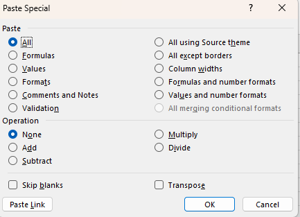
Alt + E + S – Paste Special This allows you to select how you’d like the cell(s) you’ve selected to be pasted.

Extend selection to the edge of data – These shortcuts help you maneuver in your workbooks without scrolling:
- Shift + Control + Right arrow – Select right
- Shift + Control + Left arrow – Select left
- Shift + Control + Up arrow – Select up
- Shift + Control + Down arrow – Select down
Tip 2: Advanced Filters
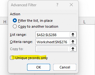
When filtering within Excel, you can use advanced filters that allow for multiple criteria sets. This feature is particularly useful for analyzing financial data and creating dashboards.
One useful advanced filter is the unique records box, which removes duplicate lines through your filter.

You also have the ability to select a criteria range to filter your data by. This allows you to filter by several criteria at once such as all sales in 2024 greater than a certain amount, or all sales in 2024 greater than a certain amount in a certain business segment.
Tip 3: Conditional Formatting
Conditional formatting is a powerful tool for presenting data clearly. Options include:
- Highlight Cells Rules – Format data based on specific conditions
- Top Bottom Rules – Identify top and bottom performers
- Data Bars and Color Scales – Create quick visualizations
- Icon Sets – Apply directional indicators

For accountants, conditional formatting can be especially useful when creating templates for:
- Budget variance analysis
- KPI tracking
- Expense monitoring
- Aging reports
Tip 4: What-If Analysis
What-if analysis is a useful tool in Excel used to calculate the outcome of multiple variables by changing one of the input values. This tip is useful when trying to calculate the break-even analysis or number of sales needed to reach a certain profit goal.
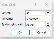
To use what-if analysis you first need to navigate to the data tab in excel and click the what-if analysis dropdown and select goal seek.

Once you’ve done this you can set a particular cell to the value you are trying to calculate to, in this case $100,000, by changing the variables that feed into that calculation, in this case A3:A5.

Tip 5: SUMIF and SUMIFS
Sum-if formulas allow you to sum cells in a data set that meet a single condition. If you need to search for cells that have multiple conditions you can use a sum-ifs function.
To use a sum-if function you first can select the range of criteria you are basing your search off of. This could be a listing of states, salespeople, dates, etc.
Once you’ve selected the range, you then need to select the corresponding criteria. In the state example you could set the criteria to “North Carolina” to sum all of the data with that data label.
After you’ve selected your criteria, you then must select the sum range. In this particular example we are selecting all of the sales revenue from the state of North Carolina.
=SUMIF(range, criteria, sum range)
=SUMIF(A1:A1000, “North Carolina”, C1:C1000)
Tip 6: IRR (Internal Rate of Return)
When evaluating a potential investment, Excel’s IRR function helps calculate your internal rate of return. This is crucial for making capital investing and budgeting decisions, allowing you to calculate project profitability and compare it to your weighted average cost of capital (WACC).
To calculate your IRR all you need is the projected cash flow of a particular project. An example could be.
Year 0 – ($1,000,000)
Year 1 – $100,000
Year 2 – $500,000
Year 3 – $1,000,000
Year 4 – $2,000,000
This particular dataset of information in Excel would calculate a 49% IRR.

Stop exporting data manually. Sync data from your business systems into Google Sheets or Excel with Coefficient and set it on a refresh schedule.
Get Started
Tip 7: NPV (Net Present Value)
Similar to IRR, when evaluating a potential investment, Excel allows you to calculate your net present value (NPV). This is important for making capital investing and budgeting decisions and gives you the NPV in terms of dollars of a potential investment, instead of a % like your IRR.
In order to calculate your NPV you will need your internal discount rate or WACC that you will discount back future payments.
Using the dataset below to calculate a NPV, assuming a 15% internal discount rate, you get a NPV of $1,100,913.98. This would indicate that you should invest in this particular project, because it has a NPV above $0.
Year 0 – ($1,000,000)
Year 1 – $100,000
Year 2 – $500,000
Year 3 – $1,000,000
Year 4 – $2,000,000
Tip 8: VLOOKUP and Advanced Lookup Functions
Lookup functions are essential for any accountant working with large dataset
The VLOOKUP function in Excel helps you pull data from one part of the same or a different spreadsheet and display it elsewhere on the spreadsheet based on the criteria selected.
For example you may be trying to run a VLOOKUP to pull in the name of each employee based on their employee ID number. Below is an example of what the VLOOKUP function would look like in Excel.
In this particular example, you would be looking at cell A2 (employee ID number), from Sheet 1 columns A through D, the employees name is in column D or the 4th column, and it needs to be an exact match so you would select FALSE instead of TRUE.
=VLOOKUP(A2,Sheet1!A:D,4,FALSE)
Once you’ve created this formula it can be copied down the spreadsheet to pull in the employee name for every employee ID number in the dataset.
Advanced Excel Features for Financial Analysis
To further enhance your accounting system, consider implementing these advanced features:
Automated Reporting with Macros
Macros can automate repetitive tasks such as:
- Monthly closing procedures
- Report generation
- Data consolidation
- Financial statements preparation
Dynamic Analysis with Pivot Tables
Excel pivot tables are powerful tools for:
- Sales analysis
- Expense tracking
- Budget vs. actual comparison
- Creating dynamic dashboards
Data Validation and Control
Implementing proper data validation helps:
- Maintain data accuracy
- Standardize inputs
- Prevent errors
- Streamline workflow
Power BI Integration
Power BI integration with Excel enables:
- Advanced analytics
- Real-time reporting
- Interactive visualizations
- Automated data refresh
Additional Tips for Accounting Professionals
For enhanced productivity, consider:
- Using subtotals for quick summaries
- Creating custom templates for recurring reports
- Implementing data validation rules
- Setting up automated cash flow tracking
Excel Tips & Tricks for Accountants
Excel has several tips and tricks that can be used to help make life easier for accountants or increase their capability at work. In this guide, there are several tips and tricks that will help you going forward, along with many more that this guide doesn’t cover. All of these tips and tricks can be used in Coefficient to make your Excel data even easier to analyze.
Ready to take your data analysis to the next level?
Try Coefficient to seamlessly integrate your Excel with live data from various business systems, enabling real-time analysis and more advanced financial modeling.

